event_functions.livemd

Using Event Functions with Integrator (and different Nx backends)

Section

# Uncomment one of the following backends: 

nx_backend = :binary
# nx_backend = :emlx
# nx_backend = :exla
# nx_backend = :torchx
# Note that if you enable :torchx you also need to add a Livebook environment variable `PATH` 
# which points to the directory which contains cmake (e.g., do `which cmake` and then add that 
# directory to `PATH`). In Livebook, go to Settings -> Environment Variables

apple_arm64? = :os.type() == {:unix, :darwin} and :erlang.system_info(:system_architecture) |> List.starts_with?(~c"aarch64")

deps = [
  {:integrator, github: "woodward/integrator"},
  {:kino_vega_lite, "~> 0.1"}
]


{deps, config} =
  case nx_backend do
    :binary -> {deps, []}
    :torchx -> {deps ++ [{:torchx, "~> 0.9.2"}], [torchx: [is_apple_arm64: apple_arm64?, add_backend_on_inspect: true]]}
    :exla -> {deps ++ [{:exla, "~> 0.9.2"}], [exla: [default_client: :host, is_mac_arm: apple_arm64?]]}
    :emlx -> {deps ++ [{:emlx, github: "elixir-nx/emlx"}], []}
  end

Mix.install(deps, config: config)

case nx_backend do
  :binary ->
    Nx.global_default_backend(Nx.BinaryBackend)

  :torchx ->
    Nx.global_default_backend(Torchx.Backend)
    # Note that Torchx does not have its own compiler!
    # It uses `Nx.Defn.Evaluator` as the compiler

  :exla ->
    Nx.global_default_backend(EXLA.Backend)
    Nx.Defn.global_default_options(compiler: EXLA)

  :emlx ->
    Nx.default_backend(EMLX.Backend)
    Nx.Defn.default_options(compiler: EMLX)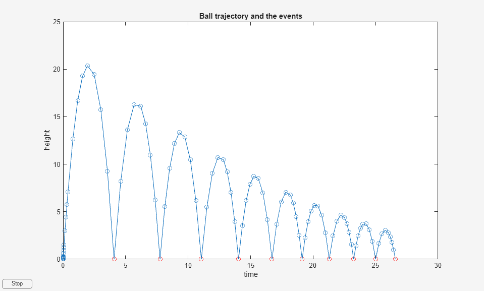
end

Usage

An event function lets you terminate a simulation based on some event (such as a collision). For this example, we're going to mimic the Matlab ballode.m bouncing ball example. See also here.

The equations of a bouncing ball are:

$$ x_0 = x_1 $$

$$ x_1 = - g $$

where $ g = 9.81 m/s^2 $. Let's encode that in an Nx function:

import Nx.Defn

alias Integrator.SampleEqns

ode_fn = &SampleEqns.falling_particle/2

The follwing event function will detect when $ x_0 $ goes negative, and will return :halt in order to terminate the simulation:

# event_fn = fn _t, x ->
#   value = Nx.to_number(x[0])
#   answer = if value <= 0.0, do: :halt, else: :continue
#   {answer, value}
# end

event_fn = &SampleEqns.falling_particle_event_fn/2

Create an empty chart to receive the data:

alias VegaLite, as: VL
alias Integrator.Point

chart =
  VL.new(
    width: 600,
    height: 400,
    title: "Bouncing Ball"
  )
  |> VL.mark(:line, point: true, tooltip: true)
  |> VL.encode_field(:x, "t", type: :quantitative)
  |> VL.encode_field(:y, "x", type: :quantitative)
  |> VL.encode_field(:color, "x_value", type: :nominal)
  |> Kino.VegaLite.new()

# |> Kino.render()

This output function will send the values of $ x_0 $ to the chart while the simulation is underway:

output_fn = fn points ->
  points = [points] |> List.flatten()

  points
  |> Enum.map(&Point.to_number(&1))
  |> Enum.map(fn point ->
    %{t: t, x: x} = point
    %{t: t, x: List.first(x), x_value: "x[0]"}
  end)
  |> Enum.map(fn point ->
    Kino.VegaLite.push(chart, point)
  end)
end

We need to define a function which will determine what to do when transitions happen, which in our case, are collisions between the ball and the ground. We'll reverse the direction of the ball, and decrease its velocity by 10% (to account for bouncing).

transition_fn = fn t, x, _multi, opts ->
  coefficient_of_restitution = -0.9
  x1 = Nx.multiply(coefficient_of_restitution, x[1])
  {:continue, t, Nx.stack([x[0], x1]), opts}
end

There's some recursive code in Integrator.MultiIntegrator that restarts the simulation when terminal events are encountered.

alias Integrator.MultiIntegrator

t_initial = Nx.f64(0.0)
t_final = Nx.f64(30.0)
x_initial = Nx.f64([0.0, 20.0])
opts = [type: :f64, output_fn: output_fn]

multi_integrator =
  MultiIntegrator.integrate(ode_fn, event_fn, transition_fn, t_initial, t_final, x_initial, opts)

Compare this plot with the version on the Matlab page: