-
-
Notifications
You must be signed in to change notification settings - Fork 1
/
Copy pathday17_land.py
181 lines (161 loc) · 6.1 KB
/
day17_land.py
1
2
3
4
5
6
7
8
9
10
11
12
13
14
15
16
17
18
19
20
21
22
23
24
25
26
27
28
29
30
31
32
33
34
35
36
37
38
39
40
41
42
43
44
45
46
47
48
49
50
51
52
53
54
55
56
57
58
59
60
61
62
63
64
65
66
67
68
69
70
71
72
73
74
75
76
77
78
79
80
81
82
83
84
85
86
87
88
89
90
91
92
93
94
95
96
97
98
99
100
101
102
103
104
105
106
107
108
109
110
111
112
113
114
115
116
117
118
119
120
121
122
123
124
125
126
127
128
129
130
131
132
133
134
135
136
137
138
139
140
141
142
143
144
145
146
147
148
149
150
151
152
153
154
155
156
157
158
159
160
161
162
163
164
165
166
167
168
169
170
171
172
173
174
175
176
177
178
179
180
181
# -*- coding: utf-8 -*-
# ---
# jupyter:
# jupytext:
# formats: ipynb,py:hydrogen
# text_representation:
# extension: .py
# format_name: hydrogen
# format_version: '1.3'
# jupytext_version: 1.9.1
# kernelspec:
# display_name: Python 3 (ipykernel)
# language: python
# name: python3
# ---
# %% [markdown]
# # Day 17 : Land
#
# Land, landcover, landuse... You choose.
# %%
import zipfile
import laspy
import pandas as pd
import pygmt
import rioxarray.merge
import xarray as xr
laspy.LazBackend.detect_available()
# %% [markdown]
# # Download and process Wellington City LiDAR into a DSM
#
# Getting the LAZ files from OpenTopography,
# do some preprocessing of the point cloud,
# and produce a Digital Surface Elevation (DSM) model.
#
# - OpenTopography link: https://doi.org/10.5069/G9K935QX
# - Bulk download location: https://opentopography.s3.sdsc.edu/minio/pc-bulk/NZ19_Wellington
#
# Code adapted from
# https://github.com/GenericMappingTools/foss4g2019oceania/blob/v1/3_lidar_to_surface.ipynb
# %%
# Download LiDAR LAZ files from a list of URLs
lazfiles: list = [
"CL2_BQ31_2019_1000_2128.laz",
"CL2_BQ31_2019_1000_2129.laz",
"CL2_BQ31_2019_1000_2130.laz",
"CL2_BQ31_2019_1000_2131.laz",
"CL2_BQ31_2019_1000_2228.laz",
"CL2_BQ31_2019_1000_2229.laz",
"CL2_BQ31_2019_1000_2230.laz",
"CL2_BQ31_2019_1000_2231.laz",
"CL2_BQ31_2019_1000_2328.laz",
"CL2_BQ31_2019_1000_2329.laz",
"CL2_BQ31_2019_1000_2330.laz",
"CL2_BQ31_2019_1000_2331.laz",
"CL2_BQ31_2019_1000_2428.laz",
"CL2_BQ31_2019_1000_2429.laz",
"CL2_BQ31_2019_1000_2430.laz",
"CL2_BQ31_2019_1000_2431.laz",
]
urls: list = [
f"https://opentopography.s3.sdsc.edu/pc-bulk/NZ19_Wellington/{lazfile}"
for lazfile in lazfiles
]
_ = pygmt.which(fname=" ".join(urls), download=True)
# %%
# Preprocess LiDAR data using blockmedian
for lazfile in lazfiles:
lazdata = laspy.read(source=lazfile)
_df = pd.DataFrame(
data={
"x": lazdata.x.scaled_array(),
"y": lazdata.y.scaled_array(),
"z": lazdata.z.scaled_array(),
}
)
# Trim the LiDAR points using blockmedian,
# and save the XYZ output to a txt file
region = pygmt.info(data=_df, spacing=5) # West, East, South, North
pygmt.blockmedian(
data=_df[["x", "y", "z"]],
T=0.99, # 99th quantile, i.e. the highest point
spacing="5+e",
region=region,
outfile=lazfile.replace(".laz", ".txt"),
)
# %%
datafiles = [lazfile.replace(".laz", ".txt") for lazfile in lazfiles]
# %%
# Create a Digital Surface Elevation Model with
# a spatial resolution of 5m.
grid: xr.DataArray = pygmt.surface(
data=" ".join(datafiles),
spacing="5+e",
region=[1_744_960, 1_746_880, 5_424_000, 5_427_600],
T=0.35, # tension factor
Ll="d", # lower bound is min value
Lu="d", # upper bound is max value
)
print(grid)
# %% [markdown]
# ## Download Wellington City Rural Aerial Photos
#
# Getting some Orthophotography within the Wellington Region taken in February 2021.
# This is RGB imagery with a spatial resolution of 30cm.
#
# Link to the data at LINZ Data Service (LDS):
# - https://data.linz.govt.nz/layer/105727-wellington-03m-rural-aerial-photos-2021
#
# Specfically, we'll get two specific tiles which covers a section of
# [Zealandia](https://en.wikipedia.org/wiki/Zealandia_(wildlife_sanctuary) in Karori,
# which is an ecosanctuary in Wellington!
# - [BQ31_5000_0506](https://data.linz.govt.nz/layer/105727-wellington-03m-rural-aerial-photos-2021/data/307/?mt=Streets&l=105024%3A0%2C105025%3A0%2C105735%2C105727%3A0&lpw=650&cv=1&z=14&c=-41.30388%2C174.76068&e=-41.29005%2C174.75521%2C-41.32222%2C174.73135&sq=-41.30049%2C174.73395~layer.105735~105735_pk663&al=m&lag_f=*&lag_q=BQ31_5000_0506)
# - [BQ31_5000_0507](https://data.linz.govt.nz/layer/105727-wellington-03m-rural-aerial-photos-2021/data/324/?mt=Streets&l=105735%2C105727%3A0&lpw=650&cv=1&z=14&c=-41.30388%2C174.76068&e=-41.29005%2C174.75521%2C-41.32222%2C174.73135&sq=-41.30049%2C174.73395~layer.105735~105735_pk663&al=m&lag_f=*&lag_q=BQ31_5000_0507)
#
# You'll need to manually create a LINZ Data Service account, login, and
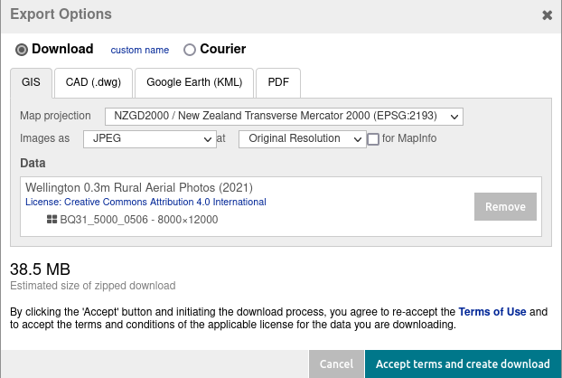
# download a zipped GeoTIFF. Choose the default EPSG:2193 projection,
# 'TIFF' as the image option, and 'Original Resolution'.
#
# 
# %%
# Unzip the files
for file in ["lds-tile-bq31-5000-0506-GTiff.zip", "lds-tile-bq31-5000-0507-GTiff.zip"]:
with zipfile.ZipFile(file=file) as z:
for zip_info in z.infolist():
z.extract(member=zip_info)
# %%
# Merge the two GeoTIFFs together into a single dataarray
rda1 = rioxarray.open_rasterio(filename="BQ31_5000_0506.tif")
rda2 = rioxarray.open_rasterio(filename="BQ31_5000_0507.tif")
rda = rioxarray.merge.merge_arrays(dataarrays=[rda1, rda2])
# %%
# Clip RGB aerial imagery to geographical extent of Zealandia sanctuary
rda_clipped = rda.rio.clip_box(
minx=1_744_960, maxx=1_746_880, miny=5_424_000, maxy=5_427_600
)
rda_clipped.rio.to_raster(raster_path="BQ31_5000_0506-0507.tif", dtype="uint8")
# %%
# Inspect the metadata of the merged GeoTIFF file
print(pygmt.grdinfo(grid="BQ31_5000_0506-0507.tif"))
# %% [markdown]
# ## Plot the map!
#
# Let's make a 3D perspective map using PyGMT's
# [`grdview`](https://www.pygmt.org/v0.5.0/api/generated/pygmt.Figure.grdview.html).
# The DSM is used as the relief grid, and draped on top is the aerial imagery.
# %%
fig = pygmt.Figure()
with pygmt.config(PS_PAGE_COLOR="black"):
fig.grdview(
grid=grid, # Digital Surface Elevation model
drapegrid="BQ31_5000_0506-0507.tif", # Aerial imagery layer
# Crop out some of the edges of the original region
# region=[1_744_960, 1_746_880, 5_424_000, 5_427_600],
region=[1_745_000, 1_746_000, 5_425_000, 5_427_000],
surftype="i280", # image draping with 280dpi resolution
perspective=[60, 45], # view azimuth and angle
zscale="0.01", # vertical exaggeration
# frame="af",
)
fig.savefig(fname="day17_land.png")
fig.show()