The goals / steps of this project are the following:
- Compute the camera calibration matrix and distortion coefficients given a set of chessboard images.
- Apply a distortion correction to raw images.
- Use color transforms, gradients, etc., to create a thresholded binary image.
- Apply a perspective transform to rectify binary image ("birds-eye view").
- Detect lane pixels and fit to find the lane boundary.
- Determine the curvature of the lane and vehicle position with respect to center.
- Warp the detected lane boundaries back onto the original image.
- Output visual display of the lane boundaries and numerical estimation of lane curvature and vehicle position.
Rubric Points
Here I will consider the rubric points individually and describe how I addressed each point in my implementation.
Code File - Advanced-Lane-Finding.ipynb Write up File - writeup.md
The jupyter notebook file has been documented with regards to what functionality each part of code implements.
Before moving onto any further processing on the images received from the camera, it is important that the image from the camera is not distorted. For that, the camera first has to calibrated. We use the chessboard images provided to us in the camera_cal folder for the purpose of calbration and undistortion.
1. Briefly state how you computed the camera matrix and distortion coefficients. Provide an example of a distortion corrected calibration image.
Chessboard images are used to calibrate the camera. The calibration is done using the object points which are the (x,y,z) coordinates of the chessboard corners in real world and the image points of the detected chessobard corners. This is done using the findChessboardCorners function of opencv module.
On getting the object points and the image points and the object points, we compute the calibration and distortion coefficients using the cv2.calibrateCamera() function. I applied this distortion correction to the chessboard image using the cv2.undistort() function and obtained this result:


Here is an example of distortion correction, applied on test images.


I chose to hardcode the source and destination points in the following manner:
src = np.float32([(575,464),
              (707,464),
              (258,682),
              (1049,682)])
dst = np.float32([(450,0),
              (w-450,0),
              (450,h),
              (w-450,h)])

where w is the width of the image and h is the height of the image.
This resulted in the following source and destination points:
| Source | Destination |
|---|---|
| 575, 464 | 450, 0 |
| 707, 464 | 830, 0 |
| 258, 682 | 450, 720 |
| 1049, 682 | 830, 720 |
Then getPerspectiveTransform(src, dst) function of the opencv library is used to get the transform and the inverse transform matrix.
Here's what it looks like:


We try the following color transformations:
- RGB-HSV
- RGB-HLS
- RGB-YUV
- RGB-LAB
Transformation Visualization 1

Thougts The original image has quite a bit of sunlight , hence the lanes are not very dark colored.
- RGB does an average job of detecting the lanes. The best job is done by the R channel of RGB.
- G channel of RGB detects the white lane decently.
- S channel of HSV does a decent job of detecting yellow lane, but not quite good with the white one. Same with the S channel of HLS
- L channel of HLS does a decent job at detecting the white pixels.
- U channel of YUV and B channel of LAB color spaces perform at a similar level st detecting yellow pixels.
Transformation Visualization 2

Thougts This image has a lot of noise due to noisy lighting conditions.
- RGB does a much better job when the lighting conditions are not bright.
- S channel of HSV and HLS does a decent job of detecting yellow lane, but seems vulnerable to noise.
- Y channel of YUV and R channel of RGB do a similar job at detecting lane pixels.
- U channel of YUV and B channel of LAB color spaces perform at a similar level st detecting yellow pixels.


Thoughts on sobel transformation
While the edge are detected in images by application of sobel transformation, it still leaves a lot to be desired as it doesnt seem to perform that well in noisy lighting conditions. Maybe color transformation can solve this.


Thoughts on color transformation
As we can see from the images above, S channel of HLS channel does a good job at detecting yellow lane pixels, but is vulnerable to noise. Compared to that, B channel of the LAB color space does an equally good job at detecting yellow lane pixels, and loks resistant to noise.
L channel of HLS does well at detecting white lane pixels.
##Connecting the complete pipeline
- perform distortion correction.
- perform sobel and color thresholding.
Lets visualize the difference in sobel and color thresholding.


Thoughts
Although it depends entirely on the values chosen for the threshold, from what has been chosen currently, it seems sobel thresholding seems to be picking up a lot of noise besides the lane lines as compared to only color thresholding. Lets go ahead with the color thresholding only and see what we get with that.
Now this was the interesting part, albeit time consuming!
Given this image, how can we go about fitting a polynomial on the lane pixels?
- Divide the problem into smaller problems by using smaller windows and detecting useful pixels for each window
- Once a certain number of useful pixels have been detected for that window, move onto next windoe and do tha same.
- Once useful pixels for all the windows have been detected for both the lanes, fit a polynomial using the function
np.polyfit.
Note: The base points for the starting window are found using the histogram of the binary image. The assumption is that the peaks on the histograms coorespond to the left and right lane pixels. To avoid picking any noise, we find the peaks between a certain fixed boundary.
Lane pixels from the calculated fits are found using the following formula:


Note that even though the peak resulting due to the noise at the extreme ends of the frame are greater than the lane peaks, still they are not considered due to the our criteria for considering base points for each window of not going to the extreme ends of the frame to look for peaks
The next step to use information from the previous frame for fitting polynomial on lane pixels. We use the left and the right fit obtained from the previous frame and use them for plotting the lane lines on the current frame.


5. Describe how (and identify where in your code) you calculated the radius of curvature of the lane and the position of the vehicle with respect to center.
The radius of curvature is calculated using the formula mentioned in this resource and Udacity lesson
The important point to notice is that radius if curvature is in m units and so far we have been dealing distances in pixels. So we need to come up with a maping between the two. Apparently, in y dimension, there are approximately 3.048 meters per 100 pixels and 3.7 meters per 378 pixels in the x dimension.
Also, the point where the radius of curvature is calculated has to be decided. We calculate the radius at the base of the image.
The distance from the center of the lane is calculated as the distance between the center of the lane (which is the means of left and right lane intercepts)and the position of the car. (You don't say!)


Final image Processing
- Thresholding using the function
pipeline_color. - If polynomial fit present from previous frame, use that information to plot lane lines using the function
polyfit_using_prev_fit, else use the functionlane_polyfitto find appropriate fits for lane pixels - Validate the fit obtained by calculating the difference between the left and right lanes x intercepts. The ideal distance is 350 pixels. If the difference in calculated left and right lanes is greater than 100 pixels from the 350 px width, discard those fits, else add those fits to the left and right Line class* instances
- Calculate the radius of curvature and distance from the center.
- Draw the fitted lane lines and the data onto the original image
Line Class - To store information about lane lines such as polynomial fits, best fits, radius of curvature etc, we create a separate class Line , which is instantiated twice, once for each left and right lane lines.
1. Provide a link to your final video output. Your pipeline should perform reasonably well on the entire project video (wobbly lines are ok but no catastrophic failures that would cause the car to drive off the road!).
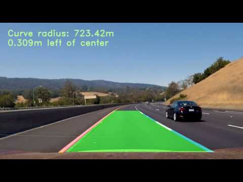
Thoughts
The pipeline words fine on the project video and looks robust on changes on lighting conditions and other noises.
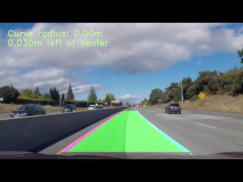
Thoughts
This one is a bit less stable. There are stretches where the pipeline breaks down completely, down to the changes in lighting conditions possibly.
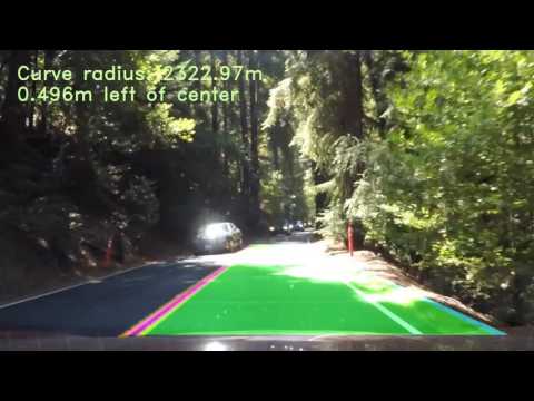
Thoughts
Well , the pipeline breaks down completely for this one. The changes in lighting are sudden, so are the changes in radius of curvature. I wouldnt want to be sitting behind the wheel with this lane finding pipeline.
1. Briefly discuss any problems / issues you faced in your implementation of this project. Where will your pipeline likely fail? What could you do to make it more robust?
The pipeline is likely to (and infact does) fail on the harder challenge video. The implementation doesnt work that well on the harder challange video. Infact, it doesnt work at all. Diagnosis shows problems with the :
1. Region of interest coordinates calculation doesnt work well enough.
The implementation for calculating region of interest could be made more robust by moving away from hard coding and coming up with a calculation scheme that takes into account the parameters of the image received such as center, width , height more effectively.
2. Thresholding doesnt work that well either.
Abrupt changes in light conditions breaks the color thresholding and a lot of noise is picked up from the surroundings. Coming up with better threshold values can make it more robust.
3. Sudden changes in radius of curvature throws off the lane finding pipeline.
To make it more robust:
- We could try fiddling with the threshold values a bit more.
- We could try improving the implementation for finding the region of interest.
- We could try to make polynomial fitting implementation more robust by accomodating for scenarios where the changes in radius of curvature are sudden.