Authors: Andrés Aldana, Michael Sebek, Gordana Ispirova, Rodrigo Dorantes-Gilardi, Giulia Menichetti (giulia.menichetti@channing.harvard.edu)
Network medicine is a post-genomic discipline that harnesses network science principles to analyze the intricate interactions within biological systems, viewing diseases as localized disruptions in networks of genes, proteins, and other molecular entities 1.
The structure of the biological network plays an essential role in the system’s ability to efficiently propagate signals and withstand random failures. Consequently, most analyses in Network Medicine focus on quantifying the efficiency of the communication between different regions of the interactome or protein-protein interaction network.
NetMedPy evaluates network localization (statistical analysis of the largest connected component/subgraph or LCC) 2, calculates proximity 3 and separation 2 between biological entities, and conducts screenings involving a large number of diseases and drug targets. NetMedPy extends the traditional Network Medicine analyses by providing four default network metrics (shortest paths, random walk, biased random walk, communicability) and four null models (perfect degree match, degree logarithmic binning, strength logarithmic binning, uniform). The user is allowed to introduce custom metrics and null models.
The pipeline workflow is depicted in the figure below.
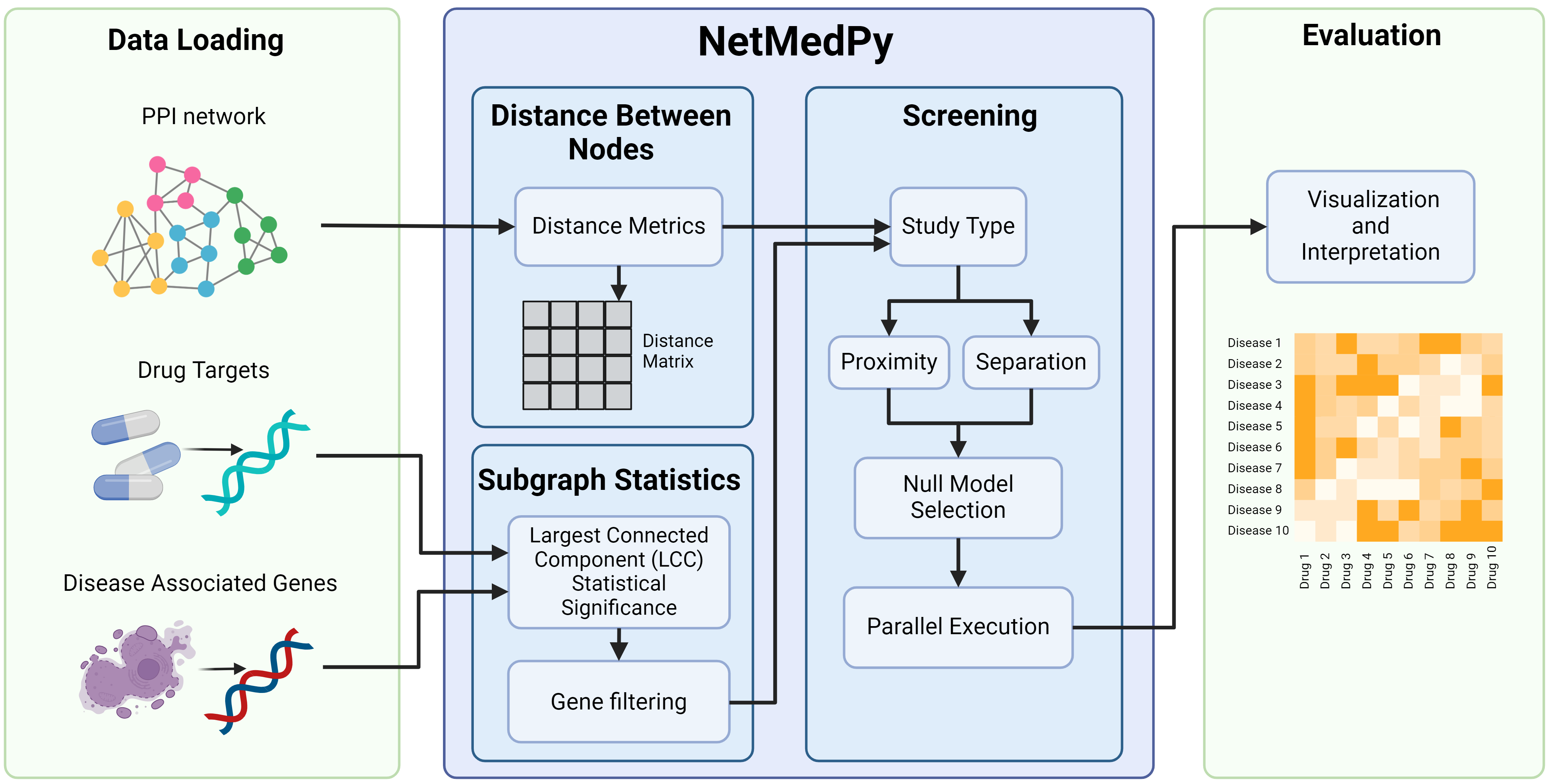
This Python implementation uses precomputed distance matrices to optimize calculations. With precalculated distances between every node pair, the code can rapidly compute proximity and separation.
NetMedPy has specific requirements for compatibility and ease of use.
NetMedPy requires Python 3.8 or newer, but it is not compatible with Python 3.12 due to incompatibility with Ray. Ensure your Python version is between 3.8 and 3.11.9 inclusive.
The following Python packages are required to run NetMedPy:
- Python (>= 3.8, <= 3.11.9)
- numpy
- pandas
- ray
- networkx
- scipy
- matplotlib
- seaborn
Users can install NetMedPy and its dependencies using PIP (recommended). Alternatively, the source code can be downloaded, allowing for manual installation of the required dependencies if more customization is needed.
While not essential, we recommend creating a dedicated conda environment for NetMedPy to ensure all dependencies are properly isolated.
Working with Conda is recommended, but it is not essential. If you choose to work with Conda, these are the steps you need to take:
-
Ensure you have Conda installed.
-
Download the environment.yml and navigate to the directory of your local/remote machine where the file is located.
-
Create a new conda environment with the
environment.ymlfile:conda env create -f environment.yml
-
Activate your new conda environment:
conda activate netmedpy_environment
Alternatively, you can install the package with PIP (in an existing conda environment, or no conda environment).
-
Ensure the following dependencies are installed before proceeding:
pip install networkx seaborn matplotlib numpy pandas ray scipy
-
Install the package:
pip install netmedpy
If none of the previous options worked, the package can be installed directly from the source code.
-
Ensure you have Python >= 3.8, <= 3.11.9 installed.
-
Copy the project to your local or remote machine:
git clone https://github.com/menicgiulia/NetMedPy.git- Navigate to the project directory:
cd NetMedPy-main- Installing the necessary dependencies:
Working with Conda is recommended, but it is not essential. If you choose to work with Conda, these are the steps you need to take:
-
Ensure you have Conda installed.
-
Create a new conda environment with the
environment.ymlfile:conda env create -f environment.yml
-
Activate your new conda environment:
conda activate netmedpy_environment
-
Ensure the following dependencies are installed before proceeding:
pip install networkx seaborn matplotlib numpy pandas ray scipy
-
Set up your PYTHONPATH (Replace
/user_path_to/NetMedPy-main/netmedpywith the appropriate path of the package in your local/remote machine.):On Linux/Mac:
export PYTHONPATH="/user_path_to/NetMedPy-main/netmedpy":$PYTHONPATH
On Windows shell:
set PYTHONPATH="C:\\user_path_to\\NetMedPy-main\\netmedpy";%PYTHONPATH%
On Powershell:
$env:PYTHONPATH = "C:\\user_path_to\\NetMedPy-main\\netmedpy;" + $env:PYTHONPATH
-
Download the directory
examples. -
Navigate to the directory
examples:
cd /user_path_to/examples- Run the
Basic_example.pyscript using Python 3 or higher:
python Basic_example.pyDetails about each function (what it is used for, what the input parameters are, the possible values of the input parameters, what the output is) from the pipeline are available in doc/build/html/NetMedPy.html and in the netmedpy/NetMedPy.py script in the comments before each function.
This example evaluates the role of Vitamin D in the modulation of autoimmune diseases, cardiovascular diseases and cancer from a network medicine perspective and reproduces the results presented in the paper "NetMedPy: A Python package for Large-Scale Network Medicine Screening"
The scripts for this example are located in the examples/VitaminD directory. There are two files that you can use for testing:
- A Python script:
VitD_pipeline.py - A Jupyter notebook:
VitD_pipeline.ipynb
-
Download the
examplesdirectory: If you haven't already done so, download theexamplesdirectory from the repository to your local or remote machine. This directory contains all the necessary files to run the examples. -
Prepare the Data: In the subdirectory
VitaminD/datathere are the files that contain the necessary data to execute the example, ensure the data files there. The output files will be stored in theVitaminD/outputsubdirectory. -
Navigate to the
VitaminDdirectory:
cd /user_path_to/examples/VitaminD- Run the Example:
python VitD_pipeline.py-
Make sure you have the
jupyterpackage installed.pip install jupyter
-
Start the Jupyter Kernel
a) If you are working on a local machine:
jupyter notebook --browser="browser_of_choice"Replace
browser_of_choicewith your preferred browser (e.g., chrome, firefox). The browser window should pop up automatically. If it doesn't, copy and paste the link provided in the terminal into your browser. The link should look something like this:b) If you are working on a remote machine:
jupyter notebook --no-browser
Then copy and paste the link provided in the terminal in your local browser of choice. It should look something like this:
-
Navigate to the
VitD_pipeline.ipynbin the Jupyter Notebook interface and start executing the cells.
-
From a dictionary of diseases
disease_genesthe function lcc_significance will calculate the statistical significance of the size of the Largest Connected Component (LCC) of a subgraph induced by the node setgenesin the networkppi. This function generates a null model distribution for the LCC size by resampling nodes from the network while preserving their degrees (null_model="log_binning"). The statistical significance of the observed LCC size is then determined by comparing it against this null model distribution. -
The parameter
null_modelcan bedegree_match,log_binning,uniform, orcustom(defined by the user).
#Load disease genes dictonary from the pickle file in `examples/VitaminD/data/disease_genes.pkl`
with open("examples/VitaminD/data/disease_genes.pkl","rb") as file:
  disease_genes = pickle.load(file)

lcc_size = pd.DataFrame(columns = ["disease","size","zscore","pval"])

for d,genes in disease_genes.items():
    data = netmedpy.lcc_significance(ppi, genes,
                                     null_model="log_binning",n_iter=10000)
    new_line = [d,data["lcc_size"],data["z_score"],data["p_val"]]
    lcc_size.loc[len(lcc_size.index)] = new_line

#Keep only diseases with an LCC larger than 10 and statistically significant
#Filtering the disease sets to the LCC is optional and not mandatory for the subsequent analyses
significant = lcc_size.query("size > 10 and zscore > 2 and pval<0.05")
disease_names = significant.disease
Evaluate Average Minimum Shortest Path Length (AMSPL) between Vitamin D and Inflammation and between Vitamin D and Factor IX Deficiency disease
- The function proximity calculates the proximity between two sets of nodes in a given graph based on the approach described by Guney et al., 2016. The method computes either the average minimum shortest path length (AMSPL) or its symmetrical version (SASPL) between two sets of nodes.
In this example, the function calculates the proximity between the Vitamin D targets stored in examples/VitaminD/data/vitd_targets.pkl and the disease genes from the examples/VitaminD/data/disease_genes.pkl file for the two diseases: Inflammation and Factor IX Deficiency. The null model of choice, in this case, is log_binning.
- The function returns a dictionary containing various statistics related to proximity, including:
- 'd_mu': The average distance in the randomized samples.
- 'd_sigma': The standard deviation of distances in the randomized samples.
- 'z_score': The z-score of the actual distance in relation to the randomized samples.
- 'p_value_single_tail': One-tail P-value associated with the proximity z-score
- 'p_value_double_tail': Two-tail P-value associated with the proximity z-score
- 'p_val': P-value associated with the z-score.
- 'raw_amspl': The raw average minimum shortest path length between the two sets of interest.
- 'dist': A list containing distances from each randomization iteration.
#Load PPI network
with open("examples/VitaminD/data/ppi_network.pkl","rb") as file:
  ppi = pickle.load(file)

#Load drug targets
with open("examples/VitaminD/data/vitd_targets.pkl","rb") as file:
  targets = pickle.load(file)

#Load disease genes
with open("examples/VitaminD/data/disease_genes.pkl","rb") as file:
  disease_genes = pickle.load(file)

inflammation = netmedpy.proximity(ppi, targets,
                                  dgenes["Inflammation"], sp_distance,
                                  null_model="log_binning",n_iter=10000,
                                  symmetric=False)

factorix = netmedpy.proximity(ppi, targets,
                                  dgenes["Factor IX Deficiency"], sp_distance,
                                  null_model="log_binning",n_iter=10000,
                                  symmetric=False)

plot_histograms(inflammation, factorix)-
The function
all_pair_distancescalculates distances between every pair of nodes in a graph according to the specified method and returns a DistanceMatrix object. This function supports multiple distance calculation methods, including shortest path, various types of random walks, and user-defined methods. -
The function
screeningscreens for relationships between sets of source and target nodes within a given network, evaluating proximity or separation. This function facilitates drug repurposing and other network medicine applications by allowing the assessment of network-based relationships. -
In this example using the
all_pair_distancesfunction the distance between every pair of nodes in the protein-protein interaction network stored in the fileexamples/VitaminD/data/ppi_network.pklare calculated, using different parameters for the method of calculation:random_walk,biased_random_walk, andcommunicability. -
For each calculation of the distance matrix the AMSPL is calculated using the
screeningfunction evaluatingproximity.
#Load PPI network
with open("examples/VitaminD/data/ppi_network.pkl","rb") as file:
  ppi = pickle.load(file)

#Load drug targets
with open("examples/VitaminD/data/vitd_targets.pkl","rb") as file:
  targets = pickle.load(file)

#Load disease genes
with open("examples/VitaminD/data/disease_genes.pkl","rb") as file:
  disease_genes = pickle.load(file)

#Shortest Paths
amspl = {"Shortest Path":screen_data["raw_amspl"]}

#Random Walks
sp_distance = netmedpy.all_pair_distances(ppi,distance="random_walk")
screen_data = netmedpy.screening(vit_d, dgenes, ppi,
                                 sp_distance,score="proximity",
                                 properties=["raw_amspl"],
                                 null_model="log_binning",
                                 n_iter=10,n_procs=20)

amspl["Random Walks"] = screen_data["raw_amspl"]

#Biased Random Walks
sp_distance = netmedpy.all_pair_distances(ppi,distance="biased_random_walk")
screen_data = netmedpy.screening(vit_d, dgenes, ppi,
                                 sp_distance,score="proximity",
                                 properties=["raw_amspl"],
                                 null_model="log_binning",
                                 n_iter=10,n_procs=20)

amspl["Biased Random Walks"] = screen_data["raw_amspl"]


#Communicability
sp_distance = netmedpy.all_pair_distances(ppi,distance="communicability")
screen_data = netmedpy.screening(vit_d, dgenes, ppi,
                                 sp_distance,score="proximity",
                                 properties=["raw_amspl"],
                                 null_model="log_binning",
                                 n_iter=10,n_procs=20)

amspl["Communicability"] = screen_data["raw_amspl"]This notebook evaluates the robustness of network-based proximity calculations between Vitamin D targets and disease-associated genes.
The objective is to assess how perturbations in the input data—such as different Protein-Protein Interaction (PPI) networks, disease-associated genes, and Vitamin D targets—impact the results obtained in the previous case study.
Before running the PPI robustness analysis, you need to download and preprocess both the PPI networks and the Vitamin D target list. This is done in three steps:
1. Download and preprocess PPI networks
For this step, we use the examples/VitaminD/supplementary/sup_code/data_integration/BioNets.ipynb notebook and the BioNetTools.py module, which provides helper functions to fetch raw PPI files from BioGrid and STRING databases (MITAB, gz, or zip), extract them, convert to a pandas DataFrame, and dump out ready‑to‑use network CSVs.
All processed networks will end up in xamples/VitaminD/supplementary/sup_data/alternative_ppi/.
2. Vitamin D targets
Use the same Vitamin D targets as in the main Vitamin D pipeline, shown in the previous example.
These targets are generated by examples/VitaminD/supplementary/sup_code/data_integration/Vit_D_Targets.ipynb and stored in examples/VitaminD/data/input/drug_targets/vitd_targets_cpie.pkl.
3. Run robustness analysis
Finally, open and run all cells in examples/VitaminD/supplementary/sup_code/robustness/PPI_Robustness.ipynb. It will:
-
Load your main PPI from
examples/VitaminD/data/input/ppi/ppi_network.pkl. -
Load each alternative PPI from
examples/VitaminD/supplementary/sup_data/alternative_ppi/(e.g. ppi_biogrid.csv). -
Load the Vitamin D target list from
examples/VitaminD/data/input/drug_targets/vitd_targets_cpie.pkl. -
Load the disease-associated genes from
examples/VitaminD/data/input/disease_genes/disease_genes_merge.pkl. -
Compute and plot the network‐robustness metrics for each scenario.
This example introduces the core concepts of network medicine through a guided analysis of Vitamin D's relationship to several diseases using protein-protein interaction networks. The Jupyter notebook (examples/NetworkMedicineIntro/Intro_Network_Medicine.ipynb) provides a step-by-step workflow demonstrating how to extract, integrate and analyze biological data to uncover drug-disease relationships.
1. Download and filter STRING PPI data
The notebook first defines the URL for STRING v12 and downloads the protein-protein interaction data:
# Define the URL for the STRING PPI dataset
string_url = "https://stringdb-downloads.org/download/protein.physical.links.v12.0/9606.protein.physical.links.v12.0.txt.gz"

# Define paths for temporary files
string_gz_path = './tmp_string/string.gz'

# Download and extract STRING data
print("Downloading STRING dataset...")
tools.download_file(string_url, string_gz_path)
tools.ungz_file(string_gz_path, "./tmp_string/string_data")
It then processes the data by removing prefixes and converting Ensembl IDs to HGNC symbols:
print("Processing protein names...")
string_df["protein1"] = string_df["protein1"].str.replace("9606.", "", regex=False)
string_df["protein2"] = string_df["protein2"].str.replace("9606.", "", regex=False)

# Convert Ensembl IDs to HGNC symbols
ens_to_hgnc = tools.ensembl_to_hgnc(string_df)
string_df["HGNC1"] = string_df["protein1"].map(ens_to_hgnc)
string_df["HGNC2"] = string_df["protein2"].map(ens_to_hgnc)
Finally, it filters the network, extracts the largest connected component, and saves it:
filtered_df = string_df.query("weight > 300")
G_string = nx.from_pandas_edgelist(filtered_df, 'HGNC1', 'HGNC2', create_using=nx.Graph())

G_string = netmedpy.extract_lcc(G_string.nodes, G_string)

# Save to CSV
df_edges = nx.to_pandas_edgelist(G_string)
df_edges.to_csv("output/string_ppi_filtered.csv", index=False)
2. Extract Vitamin D targets
The notebook extracts compound-protein databases - PubChem, Chembl, STITCH, CTD, DTC, BDB, DrugBank, OTP, DrugCentral from a pre-packaged zip file for their posterior integration with CPIExtract:
# Define database directory path
data_path = "./output/cpie_Databases"

if os.path.exists(data_path):
    shutil.rmtree(data_path)

tools.unzip_file("../VitaminD/supplementary/sup_data/cpie_databases/Databases.zip", data_path)
It then loads multiple databases into memory and searches for Vitamin D (Cholecalciferol) targets:
# Store all databases in a dictionary
dbs = {
    'chembl': chembl_data,
    'bdb': BDB_data,
    'stitch': sttch_data,
    'ctd': CTD_data,
    'dtc': DTC_data,
    'db': DB_data,
    'dc': DC_data
}

# Cholecalciferol (PubChem CID: 5280795)
comp_id = 5280795

# Initialize Comp2Prot
C2P = Comp2Prot('local', dbs=dbs)

# Search for interactions
comp_dat, status = C2P.comp_interactions(input_id=comp_id)

# Extract HGNC symbols
vd_targets = {"Vitamin D": list(comp_dat.hgnc_symbol)}

# Save extracted targets
with open('./output/vd_targets.json', 'w') as f:
    json.dump(vd_targets, f)
3. Extract and filter disease gene associations
Disease-gene associations are loaded from DisGeNet files and filtered by confidence score:
# Directory containing the disease genes
dis_gene_path = "input_data/disease_genes"

disease_file_names = {
    "Huntington":"DGN_Huntington.csv",
    "Inflammation": "DGN_inflammation.csv",
    "Rickets": "DGN_Rickets.csv",
    "Vit. D deficiency": "DGN_VDdeff.csv"
}

disease_genes = {}

# Load files and filter for strong associations
for name,file_name in disease_file_names.items():
    path = dis_gene_path + "/" + file_name

    df = pd.read_csv(path)
    df = df.query("Score_gda > 0.1")

    disease_genes[name] =  list(df.Gene)

# Save file
with open('./output/disease_genes.json', 'w') as f:
    json.dump(disease_genes, f)
4. Verify network coverage
The notebook checks which disease genes and drug targets are found in the PPI network:
# Load PPI network
ppi = pd.read_csv("output/string_ppi_filtered.csv")
ppi = nx.from_pandas_edgelist(ppi, 'source', 'target', create_using=nx.Graph())

# Keep only associations existing in the PPI
nodes = set(ppi.nodes)
for name, genes in disease_genes.items():
    disease_genes[name] = set(genes) & nodes
    print(f"{name}: {len(disease_genes[name])} associations in PPI")

for name, targets in dtargets.items():
    dtargets[name] = set(targets) & nodes
    print(f"{name}: {len(dtargets[name])} targets in PPI")
5. Compute random walk distances
The notebook calculates biased random walk distances between all nodes:
# Calculate Random Walk based distance between all pair of genes
dmat = netmedpy.all_pair_distances(
    ppi,
    distance='biased_random_walk',
    reset = 0.3
)

# Save distances for further use
netmedpy.save_distances(dmat,"output/ppi_distances_BRW.pkl")
6. Calculate proximity with log-binning null model
The notebook computes proximity z-scores using the log-binning null model:
# Calculate proximity between Vitamin D targets and Diseases
proximity_lb = netmedpy.screening(
    dtargets,
    disease_genes,
    ppi,
    dmat,
    score="proximity",
    properties=["z_score"],
    null_model="log_binning",
    n_iter=10000,n_procs=10
)

zscore_lb = proximity_lb['z_score'].T
zscore_lb = zscore_lb.sort_values(by='Vitamin D')
zscore_lb
7. Repeat analysis with degree-matched null model
The same analysis is performed using the degree-match null model for comparison:
pythonproximity_dm = netmedpy.screening(
    dtargets,
    disease_genes,
    ppi,
    dmat,
    score="proximity",
    properties=["z_score"],
    null_model="degree_match",
    n_iter=10000,n_procs=10
)

zscore_dm = proximity_dm['z_score'].T
zscore_dm = zscore_dm.sort_values(by='Vitamin D')
zscore_dm
8. Compare results from both null models
Finally, the notebook combines results from both methods for comparison:
zscore_lb.columns = ["Log Binning"]
zscore_dm.columns = ["Degree Match"]

zscore = pd.merge(zscore_lb,zscore_dm, left_index=True, right_index=True)

zscore
This produces a table showing z-scores from both null models, with Vitamin D deficiency having the strongest connection to Vitamin D targets.
- STRING v12: Human protein-protein interactions downloaded directly from
stringdb-downloads.org - Compound-target databases: Collection of databases accessed from the VitaminD supplementary data folder
- DisGeNet: Disease-gene associations provided as CSV files in the
input_datafolder
After running the notebook, the following files will be created:
output/
├── string_ppi_filtered.csv    # Filtered STRING PPI network
├── vd_targets.json           # Vitamin D protein targets
├── disease_genes.json        # Disease gene sets
├── ppi_distances_BRW.pkl     # Biased random walk distance matrix
└── cpie_Databases/ # Extracted compound-protein interaction databasesRoot folder organization (init.py files removed for simplicity):
│   .gitattributes
│   .gitignore
│   LICENSE.txt                                     // License information for the package
│   README.md                                       // Package documentation
│   environment.yml                                 // yml file to create conda environment
│   setup.py                                        // Package installation script
│
├───doc                                             // Documentation directory
│   └───source                                      // Source files for documentation
│       │   DistanceMatrix.rst                      // Documentation for DistanceMatrix module
│       │   NetMedPy.rst                            // Documentation for NetMedPy module
│       │   conf.py                                 // Sphinx configuration file for documentation
│       │   index.rst                               // Main index file for documentation
│       │   Makefile                                // Make file for building documentation
│       │   make.bat                                // Batch script for building documentation on Windows
│
├───examples                                        // directory with working examples using the NetMedPy pipeline
│   │   Basic_example.py                            // python script for running a basic example to test the pipeline
│   │   Cronometer.py                               // Performance timing utility
│   │   VitD_pipeline.ipynb                         // Jupyter notebook with Vitamin D example using the NetMedPy pipeline
│   │   VitD_pipeline.py                            // python script with Vitamin D example using the NetMedPy pipeline
│   │   1_4_netsize_edges.png                       // Figure showing network size and edges relationships
│   │   1_7_prox_vd.png                             // Figure related to proximity and Vitamin D
│   │   1_8_correlation.png                         // Correlation analysis figure
│   │   2_2_deviation.png                           // Deviation analysis figure
│   │   2_3_rank_correlation_distr...               // Rank correlation distribution figure
│   │
│   ├───NetworkMedicineIntro                        // Introduction to Network Medicine examples
│   │   │   Intro_Network_Medicine.ipynb            // Jupyter notebook with intro to network medicine
│   │   │   tools.py                                // Helper tools for the analysis
│   │   │
│   │   └───input_data/disease_genes                // Disease gene data for examples
│   │           DGN_Huntington.csv                  // Huntington disease gene data
│   │           DGN_Rickets.csv                     // Rickets disease gene data
│   │           DGN_VDdeff.csv                      // Vitamin D deficiency gene data
│   │           DGN_inflammation.csv                // Inflammation gene data
│   │
│   └───VitaminD                                    // directory with Vitamin D example using the NetMedPy pipeline
│       ├───data                                    // directory with data files necessary for the Vitamin D example
│       │   └───input                               // Input data directory
│       │       ├───disease_genes                   // Disease gene data directory
│       │       │       disease_genes_merge.pkl     // Merged disease genes data
│       │       │
│       │       ├───drug_targets                    // Drug target data directory
│       │       │       vitd_targets_cpie.pkl       // Vitamin D targets data
│       │       │
│       │       └───ppi                             // Protein-protein interaction data
│       │               ppi_network.pkl             // PPI network data
│       │               Alias.csv                   // Alias mapping file
│       │
│       ├───guney                                   // Implementation of Guney's network algorithms
│       │       distances.py                        // Distance calculation functions
│       │       network.py                          // Network manipulation functions
│       │
│       ├───output                                  // directory where the output files from the Vitamin D example are saved
│       │       amspl.pkl                           // Analysis output file
│       │       d1_d2.pkl                           // Disease pairs data
│       │       inf_fix.pkl                         // Inflammation-related output
│       │       inf_hun.pkl                         // Huntington-related output
│       │       lcc_size.pkl                        // Largest connected component size data
│       │       performance_size.csv                // Performance metrics
│       │       screen.pkl                          // Screening results
│       │
│       └───supplementary                           // Supplementary materials
│           └───sup_code                            // Supplementary code
│               └───data_integration                // Data integration scripts
│
├───images                                          // directory with figures from paper
│       OverviewPipeline.png                        // pipeline flowchart figure from paper
│
└───netmedpy                                        // directory containing the python scripts that contain the functions of the NetMedPy pipeline
        DistanceMatrix.py                           // Module for distance matrix calculations
        NetMedPy.py                                 // Core NetMedPy functionality
Details about each function (what it is used for, what the input parameters are, the possible values of the input parameters, what the output is) from the pipeline are available in doc/build/html/NetMedPy.html and in the netmedpy/NetMedPy.py script in the comments before each function.
This project is licensed under the terms of the MIT license.
1 Barabási, A. L., Gulbahce, N., & Loscalzo, J. (2011). Network medicine: a network-based approach to human disease. Nature Reviews Genetics, 12(1), 56-68.DOI 10.1038/nrg2918 ↩
2 Menche, Jörg, et al. "Uncovering disease-disease relationships through the incomplete interactome." Science 347.6224 (2015). DOI 10.1126/science.1257601 ↩
3 Guney, Emre, et al. "Network-based in silico drug efficacy screening." Nature Communications 7,1 (2015). DOI 10.1038/ncomms10331 ↩