Elastic Tube MPC design
MPTplus enables the elastic tube MPC design according to: Rakovic et al., American Control Conference (2016): Elastic tube model predictive control. The elastic tube MPC design enables designing the time-varying tubes (zooming in and out), in contrast to the widely-used (time invariant) rigid tube MPC design according to: Mayne et al., Automatica (2005): Robust model predictive control of constrained linear systems with bounded disturbances, for details consult Tube MPC design.
Note: MPTplus also enables the implicit Tube MPC design according to: Rakovic, Automatica (2023): The implicit rigid tube model predictive control. The implicit formulation of Tube MPC design enables handling of the large-scale systems, see Implicit Tube MPC design.
Note:
If the value of the parameter TubeType is set to elastic, then elastic tube MPC is designed, see how to design the Elastic Tube MPC:
option = {'TubeType','elastic'} % Elastic Tube MPC design
If the value of the parameter TubeType is set to implicit, then implicit tube MPC is designed, see how to design the Implicit Tube MPC:
option = {'TubeType','implicit'} % Implicit Tube MPC design
Otherwise, by default, if the value of the parameter TubeType is set to explicit, then explicit tube MPC is designed, see how to design the Explicit Tube MPC:
option = {'TubeType','explicit'} % Explicit Tube MPC design
Example on how to construct and evaluate Elastic Tube MPC controller:
%% TUBE MPC DESIGN
% LTI system
model = ULTISystem('A', [1, 1; 0, 1], 'B', [0.5; 1], 'E', [1, 0; 0, 1]);
model.u.min = [-1];
model.u.max = [ 1];
model.x.min = [-200; -2];
model.x.max = [ 200;  2];
model.d.min = [-0.1; -0.1];
model.d.max = [ 0.1;  0.1];
% Penalty functions
model.x.penalty = QuadFunction(diag([1, 1]));
model.u.penalty = QuadFunction(diag([0.01]));
% Prediction horizon
N = 9;
% N = 3;
option = {'TubeType','elastic','soltype',1,'LQRstability',1}
elastic_MPC = TMPCController(model,N,option)
% TMPC evaluation
x0 = [ -5; -2 ]; % Initial condition
% x0 = [ -1; -1 ]; % Initial condition
u_implicit = elastic_MPC.evaluate(x0) % MPC evaluation
[ u, feasible ] = elastic_MPC.evaluate(x0) % Feasibility check
Note: If the value of the parameter LQRstability is set to 0, then no terminal penalty and terminal set are automatically computed. The user is expected to set his/her own terminal penalty and terminal set or remain empty.
For the given uncertain LTI model and prediction horizon N, enable/disable (potentially time-consuming) construction of the explicit Tube MPC controller by:
% Explicit TMPC controller construction
eMPC = iMPC.toExplicit
% TMPC evaluation
x0 = [-5; -2]; % Initial condition
u = eMPC.evaluate(x0)  % Explicit MPC evaluation
Warning: The current version of MPTplus always displays for explicit Tube MPC controller confusing information on the prediction horizon N=1, although the controller is constructed correctly for any value of N.
For the given uncertain LTI model and prediction horizon N, the closed-loop simulation of the Tube MPC controller is evaluated by:
TMPC = iMPC % Implicit Tube MPC
Nsim = 12; % Number of simulation steps
% Closed-loop data of Tube MPC
ClosedLoopData = TMPC.simulate(x0, Nsim)
% Closed-loop data of Tube MPC for any model
closed_loop_object = ClosedLoop(TMPC, model)
ClosedLoopData = closed_loop_object.simulate(x0, Nsim)
% Show results
figure(1),hold on, box on, grid on, xlabel('k'), ylabel('System states x(k)')
stairs([0:Nsim],ClosedLoopData.X(1,:))
stairs([0:Nsim],ClosedLoopData.X(2,:))
stairs([0,Nsim],[0;0],'k--')
figure(2),hold on, box on, grid on, xlabel('k'), ylabel('Control inputs u(k)')
stairs([0:Nsim-1],ClosedLoopData.U(1,:))
%% FIGURE: Closed-loop Tube MPC
figure(1)
% System state x1
subplot(3,1,1), hold on, box on, grid on
xlabel('Control steps k'), ylabel('System state x_1(k)'), title('Closed-loop Tube MPC')
stairs([0:Nsim],ClosedLoopData.X(1,:))
stairs([0,Nsim],[0;0],'k:')
legend('x_1','Location','SouthEast')
axis([0, Nsim, -7.5, 0.5])
% System state x2
subplot(3,1,2), hold on, box on, grid on
xlabel('Control steps k'), ylabel('System state x_2(k)')
stairs([0:Nsim],ClosedLoopData.X(2,:))
stairs([0,Nsim],[model.x.min(2);model.x.min(2)],'k--')
stairs([0,Nsim],[model.x.max(2);model.x.max(2)],'k-.')
stairs([0,Nsim],[0;0],'k:')
legend('x_2','x_{2,min}','x_{2,max}','Location','Best')
axis([0, Nsim, model.x.min(2)-0.5, model.x.max(2)+0.5])
% Control inputs u
subplot(3,1,3), hold on, box on, grid on
xlabel('Control steps k'), ylabel('Control inputs u(k)')
stairs([0:Nsim-1],ClosedLoopData.U(1,:))
stairs([0,Nsim-1],[model.u.min;model.u.min],'k--')
stairs([0,Nsim-1],[model.u.max;model.u.max],'k-.')
legend('u','u_{min}','u_{max}','Location','SouthWest')
axis([0, Nsim-1, model.u.min-0.1, model.u.max+0.1])
Note, the returned output of function/method simulate is not supported for the case of the expanded vector of the control inputs (u_opt,x_opt) determined by the value of option solType - {0/1}.
For the given uncertain LTI model and prediction horizon N, get (approximated) minimum robust positive invariant set (the tube), sets of the conservative state and input constraints, and plot them (if applicable):
% TMPC controller construction
iMPC = TMPCController(model,N);
% Tube
Tube = iMPC.TMPCparams.Tube
figure, Tube.plot()
% State constraints
Xconservative = iMPC.TMPCparams.Px_robust
figure, Xconservative.plot()
% Input constraints
Uconservative = iMPC.TMPCparams.Pu_robust
figure, Uconservative.plot()
% Disturbances
Wset = iMPC.TMPCparams.Pw
figure, Wset.plot()
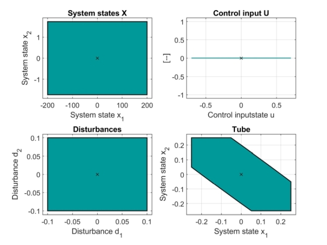
%% FIGURE: Associated sets
figure(1)
% System states
subplot(2,2,1), hold on, box on, grid on
xlabel('System state x_1'), ylabel('System state x_2'), title('System states X')
Xconservative.plot('Color',[0, 0.6, 0.6])
plot(0,0,'kx','MarkerSize',5) % origin
% Control input
subplot(2,2,2), hold on, box on, grid on
xlabel('Control inputstate u'), ylabel('[--]'), title('Control input U')
Uconservative.plot('Color',[0, 0.6, 0.6])
plot(0,0,'kx','MarkerSize',5) % origin
% Disturbances
subplot(2,2,3), hold on, box on, grid on
xlabel('Disturbance d_1'), ylabel('Disturbance d_2'), title('Disturbances')
Wset.plot('Color',[0, 0.6, 0.6])
plot(0,0,'kx','MarkerSize',5) % origin
% Tube
subplot(2,2,4), hold on, box on, grid on
xlabel('System state x_1'), ylabel('System state x_2'), title('Tube')
Tube.plot('Color',[0, 0.6, 0.6])
plot(0,0,'kx','MarkerSize',5) % origin
For the given uncertain LTI model and prediction horizon N, get the internal feedback (discrete-time LQ-optimal) controller, corresponding terminal penalty (Lyapunov) matrix, and the associated terminal set, and plot them (if applicable):
% TMPC controller construction
option = {'LQRstability',1, 'solType',1};
iMPC = TMPCController(model,N,option)
% K: u(0) = u_opt + K*( x(0) - x_opt )
K = iMPC.TMPCparams.K
% Terminal penalty: P > 0
P = iMPC.model.x.terminalPenalty.weight
% Terminal set: X_N
X_N = iMPC.model.x.terminalSet
figure, X_N.plot()
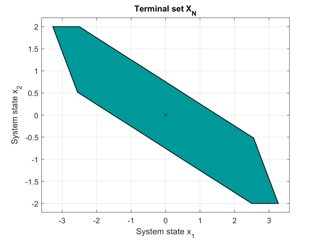
%% FIGURE: Terminal set
figure(1), hold on, box on, grid on
xlabel('System state x_1'), ylabel('System state x_2'), title('Terminal set X_N')
X_N.plot('Color',[0, 0.6, 0.6]) % Terminal set
plot(0,0,'kx','MarkerSize',5) % origin
Note: The terminal set (terminalSet) is not stored directly in the object of the system model model (ULTISystem), but the terminal set is stored in the object of the Tube MPC controller iMPC (TubeMPCController) in its parameter/property model (ULTISystem). This feature prevents misunderstanding when designing the LQR-based terminal set (for LTISystem) above the uncertain LTI system (ULTISystem).
For the given uncertain LTI model and prediction horizon N, get the associated parameters of Tube MPC design:
option = {'solType',1,'LQRstability',1}
iMPC = TMPCController(model,N,option);
% number of iterations for construction of implicit tube: Ns
Ns = iMPC.TMPCparams.Ns
% shrinking factor of implicit tube: alpha
alpha = iMPC.TMPCparams.alpha
% tolerance for evaluation of alpha: alpha_tol
alpha_tol = iMPC.TMPCparams.alpha_tol
For given feedback control law: u(0) = u_opt + K*( x(0) - x_opt ) , switch between returning the compact control input u(0) and the vector of the particular variables u_opt and x_opt using the option solType - {0/1}.
For the given uncertain LTI model and prediction horizon N, evaluate the vector of the particular variables u_opt and x_opt:
% Setup for expanded control input
option = {'TubeType','elastic','solType',0}
% TMPC controller construction
elastic_MPC = TMPCController(model,N,option)
% TMPC evaluation of expanded control input
x0 = [-5; -2]; % Initial condition
[ ux_elastic, feasible, elastic_openloop ] = elastic_MPC.evaluate(x0) % Enriched output
sigma_elastic = elastic_openloop.sigma(:,1) % SIGMA-values of the current Elastic Tube
Note, the returned output sigma_elastic represents a vector of shaping each half-space of the elastic tube (polytope) in the current control step.
Evaluation of the compact control input u(0):
% Setup for compact control input
option = {'solType',1}
% TMPC controller construction
iMPC = TMPCController(model,N,option)
% Explicit TMPC controller construction
eMPC = iMPC.toExplicit
% TMPC evaluation of compact control input
x0 = [-5; -2]; % Initial condition
ux_implicit = iMPC.evaluate(x0) % Implicit MPC evaluation
Example on how to construct and evaluate Tube MPC controller using the particular variables of the feedback control law:
% Closed-loop simulation for solType == 0
% LTI system
model = ULTISystem('A', [1, 1; 0, 1], 'B', [0.5; 1], 'E', [1, 0; 0, 1]);
model.u.min = [-1];
model.u.max = [ 1];
model.x.min = [-200; -2];
model.x.max = [ 200;  2];
model.d.min = [-0.1; -0.1];
model.d.max = [ 0.1;  0.1];
% Penalty functions
model.x.penalty = QuadFunction(diag([1, 1]));
model.u.penalty = QuadFunction(diag([0.01]));
% Prediction horizon
N = 9;
% Include the LQR-based terminal penalty and set for compact control law
option = {'TubeType','elastic', 'LQRstability',1, 'solType',0};
% Construct Tube MPC controller
elastic_MPC_expanded = TMPCController(model,N,option)
% TMPC evaluation
x0 = [ -5; -2 ]; % Initial condition
Nsim = 12; % Number of simulation steps
elastic_loop = ClosedLoop(elastic_MPC_expanded, model)
ClosedLoopData = elastic_MPC_expanded.simulate(x0, Nsim) % Implicit Tube MPC
% ClosedLoopData = eMPC_expanded.simulate(x0, Nsim) % Explicit Tube MPC
for k = 1 : Nsim, w(:,k) = elastic_MPC_expanded.TMPCparams.Pw.randomPoint; end % Fixed sequence of disturbances
ClosedLoopData = elastic_MPC_expanded.simulate(x0, Nsim, w) % Implicit Tube MPC
% ClosedLoopData = eMPC_expanded.simulate(x0, Nsim, w) % Explicit Tube MPC
figure(1),hold on, box on, grid on, xlabel('k'), ylabel('System states x(k)')
stairs([0:Nsim],ClosedLoopData.X(1,:))
stairs([0:Nsim],ClosedLoopData.X(2,:))
stairs([0,Nsim],[0;0],'k--')
figure(2),hold on, box on, grid on, xlabel('k'), ylabel('Control inputs u(k)')
stairs([0:Nsim-1],ClosedLoopData.U(1,:))

%% FIGURE: Closed-loop Tube MPC design sets
figure(1), hold on, box on, title('Closed-loop Tube MPC'), xlabel('x_1'), ylabel('x_2')
plot(ClosedLoopData.Xnominal(1,:),ClosedLoopData.Xnominal(2,:),'kx:','LineWidth', 2, 'MarkerSize', 6)
plot(ClosedLoopData.X(1,:),ClosedLoopData.X(2,:),'k*--','LineWidth', 2, 'MarkerSize', 6)
plot( elastic_MPC_expanded.model.x.terminalSet, 'Color',[0, 0.6, 0.6] )

for k = 2 : size(ClosedLoopData.Xnominal,2)
    elasticTube = Polyhedron('A', elastic_MPC_expanded.TMPCparams.Tube.A, 'b',elastic_MPC_expanded.TMPCparams.Tube.b .* ClosedLoopData.SIGMAnominal(:,k-1));
    plot( elasticTube + [ ClosedLoopData.Xnominal(:,k) ], 'Color',[0, 0.8, 0.6] )
end
plot(ClosedLoopData.Xnominal(1,:),ClosedLoopData.Xnominal(2,:),'kx:','LineWidth', 2, 'MarkerSize', 6)
plot(ClosedLoopData.X(1,:),ClosedLoopData.X(2,:),'k*--','LineWidth', 2, 'MarkerSize', 6)
legend('nominal states','uncertain states','terminal set','tube')
Example on how to set the auxiliary terminal ingredients "Pz" and "Kz" by extending the options:
% Options extended by auxiliary terminal ingredients "Pz" and "Kz":
[Kz,Pz] = dlqr(model.A,model.B,model.x.penalty.weight*10, model.u.penalty.weight);
option = {'TubeType','elastic','LQRstability',1,'Nz', 3, 'Pz', Pz, 'Kz', -Kz};
% Compute the Tube MPC object
TMPC = TMPCController(model,N,option);
% Perform simulation
x0 = [-5;-2]; % initial condition
Nsim = 15;    % number of simulation steps
ClosedLoopData = TMPC.simulate(x0,Nsim);
figure, stairs(ClosedLoopData.X')
figure, stairs(ClosedLoopData.U')

%% FIGURE: Axiliary terminal ingredients
figure(1)
% System state x1
subplot(4,1,1), hold on, box on, grid on
xlabel('Control steps k'), ylabel('System state x_1(k)'), title('Closed-loop Tube MPC')
stairs([0:Nsim],ClosedLoopData.X(1,:))
stairs([0,Nsim],[0;0],'k:')
legend('x_1','Location','SouthEast')
axis([0, Nsim, -7.5, 0.5])
% System state x2
subplot(4,1,2), hold on, box on, grid on
xlabel('Control steps k'), ylabel('System state x_2(k)')
stairs([0:Nsim],ClosedLoopData.X(2,:))
stairs([0,Nsim],[model.x.min(2);model.x.min(2)],'k--')
stairs([0,Nsim],[model.x.max(2);model.x.max(2)],'k-.')
stairs([0,Nsim],[0;0],'k:')
legend('x_2','x_{2,min}','x_{2,max}','Location','Best')
axis([0, Nsim, model.x.min(2)-0.5, model.x.max(2)+0.5])
% Control inputs u
subplot(4,1,3), hold on, box on, grid on
xlabel('Control steps k'), ylabel('Control inputs u(k)')
stairs([0:Nsim-1],ClosedLoopData.U(1,:))
stairs([0,Nsim-1],[model.u.min;model.u.min],'k--')
stairs([0,Nsim-1],[model.u.max;model.u.max],'k-.')
legend('u','u_{min}','u_{max}','Location','SouthWest')
axis([0, Nsim-1, model.u.min-0.1, model.u.max+0.1])
% Distrbance d
subplot(4,1,4), hold on, box on, grid on
xlabel('Control steps k'), ylabel('Disturbance d(k)')
stem([0:Nsim-1],ClosedLoopData.D(1,:),'filled')
stem([0:Nsim-1],ClosedLoopData.D(2,:),'filled')
stairs([0,Nsim-1],[model.d.min(1);model.d.min(1)],'k--')
stairs([0,Nsim-1],[model.d.max(1);model.d.max(1)],'k-.')
legend('d_{1}','d_{2}','Location','SouthWest')
axis([0, Nsim-1, model.d.min(1)-0.05, model.d.max(1)+0.05])