Bondora-Financial-Risk-Prediction

Credit risk modeling of peer-to-peer lending Bondora systems. Applying Data Cleaning to Bondora Raw Loans Dataset, Exploratory Data Analysis, and Visualizations for the data. Feature Engineering for the Features Set. Classifications and Regression Modeling with Pipelines, and Finally Deployment to a Web Application using Flask and Render.

This Repository is Part of the Machine Learning Engineer Internship at Technocolabs

Deployed Web App at Render: https://bondora-financial-risk-prediction.onrender.com/

Abstract

• In this project we will be doing credit risk modeling of peer-to-peer lending Bondora systems, Peer-to-peer lending has attracted considerable attention in recent years, largely because it offers a novel way of connecting borrowers and lenders. But as with other innovative approaches to doing business, there is more to it than that. Some might wonder, for example, what makes peer-to-peer lending so different–or, perhaps, so much better–than working with a bank, or why has it become popular in many parts of the world.

• Certainly, the industry has witnessed strong growth in recent years. According to Business Insider, transaction volumes in the U.S. and Europe, the world’s leading P2P markets, have expanded at double and, in some cases, triple-digit percentage rates, bolstered by widespread acceptance of doing business online and a supportive regulatory environment.

• For investors, "peer-2-peer lending," or "P2P," offers an attractive way to diversify portfolios and enhance long-term performance. When they invest through a peer-to-peer platform, they can profit from an asset class that has proven itself in both good times and bad. Equally important, they can avoid the risks associated with putting all their eggs in one basket, especially at a time when many experts believe that traditional favorites such as stocks and bonds are riskier than ever.

• Default risk has long been a significant risk factor to test borrowers’ behavior in Peer-to-Peer (P2P) lending. In P2P lending, loans are typically uncollateralized and lenders seek higher returns as compensation for the financial risk they take. In addition, they need to make decisions under information asymmetry that works in favor of the borrowers. In order to make rational decisions, lenders want to minimize the risk of default on each lending decision and realize the return that compensates for the risk.

• As in the financial research domain, there are very few datasets available that can be utilized for building and analyzing credit risk models. This dataset will help the research community in building and performing research in the credit risk domain.

Understanding the Data

• Data for the study has been taken from a leading European P2P lending platform (Bondora). The retrieved data is a pool of both defaulted and non-defaulted loans from the period between 1st March 2009 and 27th January 2020. The data comprises demographic and financial information on borrowers and loan transactions. In P2P lending, loans are typically uncollateralized and lenders seek higher returns as compensation for the financial risk they take. In addition, they need to make decisions under information asymmetry that works in favor of the borrowers. In order to make rational decisions, lenders want to minimize the risk of default on each lending decision and realize the return that compensates for the risk.

• Dataset Attributes Definitions Can be Found Here

Initial Data Preprocessing

• From the first look at the data we knew that we have a huge dataset with (134529, 112) rows and columns, a huge number of the rows had null values, so we decided to drop firstly the features that had more than 40% of null values, decreasing the number of features to 77 feature, then drop some features which will have no role in default prediction, so we managed to get the data to have 48 relevant features,

• After some cleaning we moved to Creating Target Variable for the Classification of Loan Status

  • Here, status is the variable that helps us in creating the target variable. The reason for not making status as target variable is that it has three unique values current, Late, and repaid. There is no default feature but there is a feature default date which tells us when the borrower has defaulted means on which date the borrower defaulted. So, we will be combining Status and Default date features for creating the target variable. The reason we cannot simply treat Late as default is that it also has some records in which the actual status is Late but the user has never defaulted i.e., the default date is null. So we will first filter out all the current status records because they are not matured yet they are current loans.

• Now with checking the datatypes for features and searching for any data type mismatch

  • First, we will delete all the features related to the date as it is not a time series analysis so these features will not help in predicting the target variable.
  • many columns are present as numeric but actually they are categorical as per their data description So we will convert these features to categorical features with proper mapping to their categories.

• Finally after preprocessing and cleaning the data we can continue with EDA.

• You Can refer to these steps in the Preprocessing Notebook

Exploratory Data Analysis

• First of all, we need to perform data cleaning and fill in all the null values, we separated the categorical features and filled the null values in it with the Mode, and for the Numerical Features, we fill it with the Mean. and dropped unwanted string-type columns.

Visualizing the missing values

• Now we are ready for visualizing the data, Most of the Features were highly positively right skewed as we can see here.

• and the categorical features had most of their categories as Not Set/Not Specified like some of these features.

• Also most of the features suffer from a high percentage of outliers as per these features.

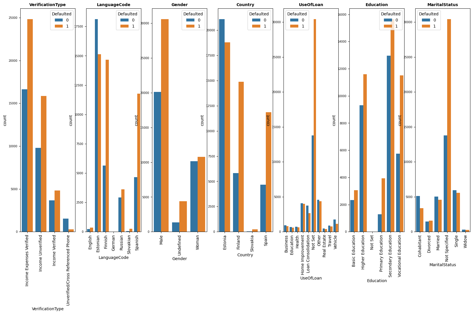
• But we had interesting insights about the data we can find here, like most of the borrowers are males whose marital status is not specified, and most of them are from Estonia with secondary education not specifying the use of the loan.

• Let's have a look at the insights between features and the target variable, as expected most of the accepted loans are for males but with more acceptance rates from Spain and Finland for secondary and vocational education borrowers.

• Also interesting insights are that most of the accepted loans are for higher-age borrowers and most of the loans are in a small range of up to 4000.

• Now, Let's have a look at the correlation between features and the target variable.

Looks like our Target Variable has a strong linear relationship with PrincipalBalance which is a highly positive correlation, and a highly negative correlation with PrincipalPaymentsMade, Also we can say low positive correlation with InterestAndPenaltyBalance

• And a look at the correlation matrix for the whole data

Looks like these features are highly positively correlated with each other

AppliedAmount, Amount, MonthlyPayment, PrincipalBalance

ExistingLiabilities, NoOfPreviousLoansBeforeLoan, AmountOfPreviousLoansBeforeLoan

PrincipalPaymentsMade, BidsPortfolioManager, InterestAndPenaltyPaymentsMade

Also Looks like NewCreditCustomer Columns are highly negatively correlated with these features

NewCreditCustomer ----> AmountOfPreviousLoansBeforeLoan, ExistingLiabilities, NoOfPreviousLoansBeforeLoan

• You Can See Far more Insights in the EDA Notebook

Feature Engineering

• Starting with the Mutual information selection between features and target variable, To detect any kind of relationship, Unlike correlation that can only detect linear relationships.

We can that the top 3 features are the ones that have a high correlation with the target variables.

• Let's fast-check the model performance to make a baseline before feature engineering

here we get 99% accuracy without any feature engineering using a random forest classifier. obviously, it is overfitting the top 3 features we have which are leaky features that are made after the loan has been accepted, and due to they won't be available at deployment, we will drop those 3 features

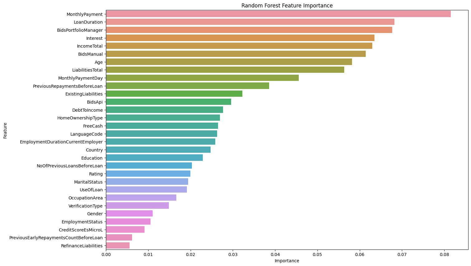
• After dropping the leaky features we get reasonable initial accuracy of 74%, with proper feature importance to most features

• Moving on, we will remove outliers with percentiles only between quantile([0.001, 0.99], resulting in decreasing number of rows from 77393 to 67314 .

• Then Encoding Categorical Features with Label Encoding using pandas factorize method.

• And Normalizing the features with Sklearn StandardScaler and transforming the features making the highly skewed features less skewed with PowerTransformer.

• Jumping on to Cluster analysis, First by finding the optimal number of clusters with the elbow method

Clustering wasn't very helpful in increasing accuracy.

• Now with PCA

  • Let's first Find the Optimum Number of Components with the elbow method

    

  • And Testing the performance with the selected 16 components of PCA, Was't very great. Only 71% Accuracy.

    

• Let's now perform Feature Selection

  • First Dropping Most Corralted Features to each other

  • Secondly using RFE (Recursive Feature Elimination) with Random Forest, Selecting the top 20 most important features

  

  Nearly no difference in Accuracy with 74% also, but with only 20 features, not 47.

• Finally, Performance Comparing for Selected Features with XGboost and Logistic Regression

  • XGBoost interestingly gave less accuracy than Random Forest 71%

  • Not so different with Logistic Regression giving about 70% Accuracy.

• You Can refer to these steps in the Feature Engineering Notebook

Classification Modeling

• We know that our current accuracy is 74% with random forest using 20 features after feature engineering.

• We will use two models in the classification part RandomForestClassifier and LogisticRegression.

• We will first make a pipeline that has the preprocessing steps StandardScaler and PowerTransformer with the random forest model and another with the logistic regression.

• Now, With the Hyper Parameters Tuning

  • First, trying grid search with 3 different values of hyperparameters for Random Forest: n_estimators, max_features, max_depth, min_samples_split, min_samples_leaf, and penalty, C, Solver for Logistic Regression, Resulting in not very increase in accuracy with Random Forest and in a slight increase 70% with Logistic Regression.
  • Secondly with Randomized Search with more range in values for the same hyperparameters, resulting in a slight increase in accuracy of 75% with Random Forest. But the same accuracy with Logistic Regression.

• Let's Proceed with Model Evaluation

  • with Random Forest Roc Auc Score was 80%

    

    

    with Classification Matrix for Random Forest Model We can see the Model Struggling with the Not Defaulted Class.

  • with Logistic Regression Roc Auc Score was only 70%

  

  

  with Classification Matrix for Logistic Regression We can see the Model also Struggling with the Not Defaulted Class.

• We will proceed with the Random Forest Model due to its better accuracy (75%).

• You Can refer to these steps in the Classification Modeling Notebook

Regression Modeling

• for the Regression Part we have three Target variables

  • Preferred EMI (Monthly Payment)
  • Repayment Years (Should be able to pay the loan for that period)
  • ROI (Return on Investment)

• We will first Create these Features

  • EMI = [P x R x (1+R)^N]/[(1+R)^N-1], where P stands for the loan amount or principal, R is the interest rate per month [if the interest rate per annum is 11%, then the rate of interest will be 11/(12 x 100)], and N is the number of monthly installments. Using Amount, Interest, LoanDuration Features
  • ROI = Investment Gain / Investment Base , ROI = Amount lended * interest/100

  ROI = Interest Amount / Total Amount. Creating First InterestAmount, TotalAmount.

  • Repayment Years: Calculating how many months to pay the full total amount of the loans, then dividing it to be years.

• After Creating the 3 Target Variables we will try Linear Regression and Adaboost Regressor Models

• with Linear Regression the Accuracy was not that bad.

  • giving 66% for Repayment Years
  • Interestingly giving 86% for EMI
  • giving 95% for ROI

• with Adaboost Regressor the Accuracy was far better.

  • giving 86% for Repayment Years
  • Interestingly giving 84% for EMI
  • giving 99% for ROI

• We will proceed with the Adaboost Regressor due to its better accuracy in the 3 Target Variables.

• You Can refer to these steps in the Regression Modeling Notebook

Making Piplines

• First, we will save the trained models in pickle files to load them fast when we make the web application with Flask

• For the Classification Model Random Forest Model Size was above 100MB, So we had to compress it with Joblib Library, Making it about 20MB.

• and for Regression Model we saved the three Adaboost Regressor Models trained on separate target variables.

• Also Saving the Preprocessing Pipeline to Transform new Prediction Data.

• Then We Proceed to make one prediction function that takes as an input the 20 features we selected in the Feature Engineering Part.

• The Prediction Function had

  • Process input data, and handle their datatypes to the same as the original trained data.
  • Encoding Categorical Features the same way Encoded in training
  • Transforming the data with the Preprocessing Pipeline, to be in the same format the Models trained on.
  • Finally Making Predictions with the saved models.
  • Outputting a data frame that has the full four target variables

• Finally, we checked the accuracy of predicting the Whole Data

  • For the Classification Modeling, the Accuracy was pretty good about 94%.
  • For the Regression Modeling, it had a Slightly Increase in Some of the Models.

• You Can refer to these steps in the Piplines Notebook

Deployment

• We began with Making the Front End of the Web Application, Then Implementing the Prediction Function and making sure to pass the required inputs, and it's returning the proper outputs.

• After Making Sure the Web app was Running Correctly, Giving the Same Results we had Before. We Proceed with the Deployment

• We Deployed the Web App with Render.com, After Installing the Required Dependencies on the Cloud Server.

• You Can Check the Deployed Web App Here.

• You Can refer to these steps in the Deployment Branch.