df03_tidyverse.qmd

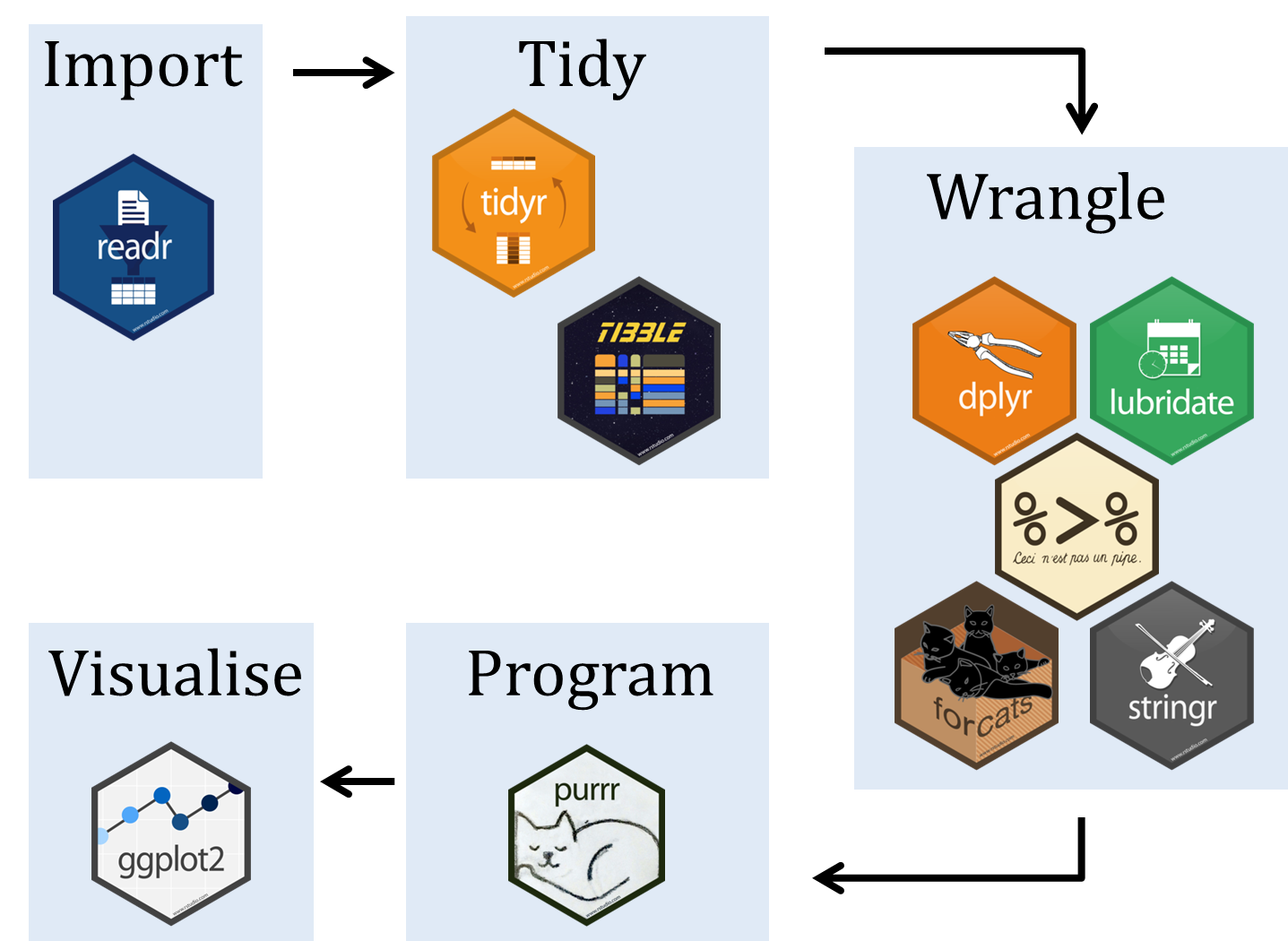
# Introduction to tidyverse

The R Tidyverse is a [collection of packages](https://www.tidyverse.org/packages/) for data handling, analysis and visualization.
If you want to use the `tidyverse`, you have to install the additional packages first with the `install.packages()` function.
Once installed, you then have to tell R to make the `tidyverse` functions available in your current R session with `library()`
You only have to install a package once, but loading it has to be done every time you start a new R session. It is recommened to either not 
include the `install.packages()` in your script or just comment it out like below.


```{r}
# install.packages("tidyverse")
library(tidyverse)
```

As you see in the output, `library(tidyverse)` actually loads nine different packages. It will also give you a warning about conflicting functions. Do not worry for now, we will get to that in time.


## Why tidyverse?


* consistent syntax and workflows
* makes code more readable
* pipe operator `%>%` / `|>` can chain functions together
* **tidy data approach**
    * rows are observations
    * columns are variables / features


![https://ajsmit.github.io/Intro_R_Official/figures/tidy_workflow.png](https://ajsmit.github.io/Intro_R_Official/figures/tidy_workflow.png)



## data.frames with dplyr

* provides functions for `data.frame` manipulation
* can complement or replace base R functions


```{r}
#| echo: false
#| fig-sub: "https://biostat2.uni.lu/lectures/img/06/vaudor_dplyr_schema.png"
knitr::include_graphics("https://biostat2.uni.lu/lectures/img/06/vaudor_dplyr_schema.png")
```


Of course, you can also load single packages from the `tidyverse` with the `library()` function.



```{r}
library(dplyr)
trees = read.csv("data/muenster_trees.csv")
```



### `slice` - a slice of data - i.e. the specified rows
```{r}
trees = slice(trees, seq(8))
```

### `select` - selects columns

```{r}
select(trees, species)
```

### `filter` - filters rows based on logical operators
```{r}
filter(trees, species == "Tilia")
```

### `mutate` - mutates the data.frame by adding columns

```{r}
mutate(trees, city = "Muenster")
```

### `summarise` - summarises data
```{r}
summarise(trees, amount = n_distinct(species))
```


### `pull` - pulls the values out of a column

```{r}
pull(trees, species)
```



Note that the functions above could all be realized with base R. Think about the tidyverse as a different dialect to data analysis with R. Later on, it will be up to you which style you like more and feels more natural to your thought process. However, for understanding code you randomly find on the internet or if you work with other people that prefer different dialects than yourself, you should be able to read and write the basics of each style regardless.

```{r}
#| eval: false
# the same in base R

# select
trees$species

# filter
trees[,trees$species == "Tilia"]

# mutate
trees$city = "Muenster"

# summarise
length(unique(trees$species))

```



## The pipe operator

The strength of dplyr is the possibility to chain functions with `%>%` or `|>`.


```{r}
trees|> 
    filter(species == "Tilia" | species == "Platanus") |> 
    pull(district) |>  
    unique()
```


With base R functions this looks messy, because we have to use functions inside functions.

```{r}
unique(trees$district[trees$species == "Tilia" | trees$species == "Platanus"])
```