


BD-rate implementations in Python. Also available in Matlab.
The Bjøntegaard-Delta (BD) metrics (delta bit rate and delta PSNR) described in [1] are well known metrics to measure the average differences between two rate-distortion (RD) curves. They are based on cubic-spline interpolation (CSI) of the RD curves and Matlab as well as Python implementations are available on the internet.
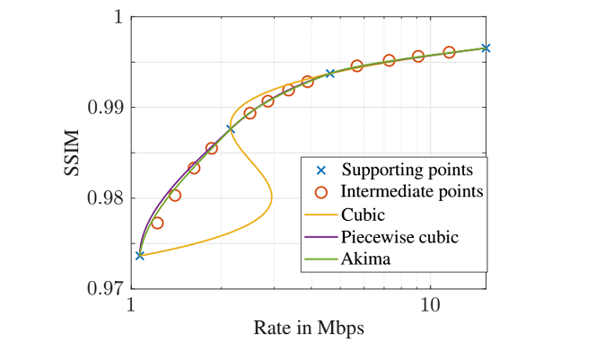
However, this way of interpolation using a third-order polynomial leads to problems for certain RD curve constellations and causes very misleading results. This has also been experienced during the standardization of HEVC. Consequently, the so-called piecewise cubic hermite interpolation (PCHIP) has been implemented in the JCT-VC Common Test Conditions (CTC) Excel sheet [2] for performance evaluation. In further studies [4] - [5], it was found that Akima interpolation returns more accurate and stable results. An example for corresponding interpolated curves is shown below.
This page provides BD-rate implementations (see here for a Matlab implementation) for both cubic-spline interpolation, PCHIP, and Akima interpolation in Python. In our tests, the implementation of PCHIP returns the same value as the Excel-Implementation from [3] with an accuracy of at least 10 decimal positions. The scripts allow to calculate the BD-rate for any number of RD points greater one.
bjontegaard is best installed via pip: pip install bjontegaard.
Basic example with test data measured using ffmpeg (libx265 with different preset settings) and Akima interpolation:
# Import the package
import bjontegaard as bd

# Test data
rate_anchor = [9487.76, 4593.60, 2486.44, 1358.24]
psnr_anchor = [ 40.037,  38.615,  36.845,  34.851]
rate_test = [9787.80, 4469.00, 2451.52, 1356.24]
psnr_test = [ 40.121,  38.651,  36.970,  34.987]

# Use the package
bd_rate = bd.bd_rate(rate_anchor, psnr_anchor, rate_test, psnr_test, method='akima')
bd_psnr = bd.bd_psnr(rate_anchor, psnr_anchor, rate_test, psnr_test, method='akima')

print(f"BD-Rate: {bd_rate:.4f} %")
print(f"BD-PSNR: {bd_psnr:.4f} dB")
This package provides two main functions for BD metric calculation:
bd_rate(rate_anchor, dist_anchor, rate_test, dist_test, method, require_matching_points=True, interpolators=False)bd_psnr(rate_anchor, dist_anchor, rate_test, dist_test, method, require_matching_points=True, interpolators=False)
The parameters rate_anchor and dist_anchor describe the rate-distortion points of the anchor, rate_test and dist_test describe the rate-distortion points of the test codec.
Available interpolation methods:
'cubic': Cubic spline interpolation'pchip': Piecewise cubic hermite interpolation (used in standardizations [2], [3])'akima': Akima interpolation [4]
If require_matching_points=True (default), the number of rate-distortion points for anchor and test must match.
If interpolators=True is given, the functions additionally return the internal interpolation objects that can be used to check the behaviour of the value interpolation.
For in-depth evaluation of codec comparison results, we recommend to take relative curve difference plots (RCD-plots) into account (see [5]). They can be created using:
plot_rcd(rate_anchor, dist_anchor, rate_test, dist_test, method, require_matching_points=True, samples=1000)
Here is an example for a RCD plot.

The left plot shows the supporting points and the Akima-interpolated curves for both anchor and test. The right plot shows the relative horizontal difference between the two curves in percentage.
The function compare_methods generates a plot that compares the internal interpolation behaviour of the three variants.
The parameters rate_label, distortion_label, and figure_label control the figure and axis labels of the plot.
If filepath is given, the final figure is saved to this file.
import bjontegaard as bd

# Test data
rate_anchor = [9487.76, 4593.60, 2486.44, 1358.24]
psnr_anchor = [ 40.037,  38.615,  36.845,  34.851]
rate_test = [9787.80, 4469.00, 2451.52, 1356.24]
psnr_test = [ 40.121,  38.651,  36.970,  34.987]

# Compare the internal behaviour of the three variants
bd.compare_methods(rate_anchor, psnr_anchor, rate_test, psnr_test, rate_label="Rate", distortion_label="PSNR", figure_label="Test 1", filepath=None)
Furthermore, a comparison between the interpolated curves and intermediate, true rate-distortion points between the supporting points is shown in the plot below. For this example, the quality is represented by the SSIM value. Note that the example was cherry-picked to show that cubic interpolation can fail. The curve interpolated by the Akima interpolator is closest to the intermediate points.
[1] G. Bjontegaard, "Calculation of average PSNR differences between RD-curves", VCEG-M33, Austin, TX, USA, April 2001.
[2] F. Bossen, "Common HM test conditions and software reference configurations", JCTVC-L1100, Geneva, Switzerland, April 2013.
[3] F. Bossen, "VTM common test conditions and software reference configurations for SDR video", JVET-T2020, Teleconference, October 2020.
[4] C. Herglotz, M. Kränzler, R. Mons, A. Kaup, "Beyond Bjontegaard: Limits of Video Compression Performance Comparisons", Proc. International Conference on Image Processing (ICIP) 2022, online available.
[5] C. Herglotz, H. Och, A. Meyer, G. Ramasubbu, L. Eichermüller, M. Kränzler, F. Brand, K. Fischer, D. T. Nguyen, A. Regensky, and A. Kaup, “The Bjøntegaard Bible – Why Your Way of Comparing Video Codecs May Be Wrong,” IEEE Transactions on Image Processing, 2024, online available.
BSD 3-Clause. For details, see LICENSE.