README.Rmd

---
output: github_document
---

<!-- README.md is generated from README.Rmd. Please edit that file -->
<!-- devtools::rmarkdown::render("README.Rmd") -->
<!-- Rscript -e "library(knitr); knit('README.Rmd')" -->

```{r, echo = FALSE}
knitr::opts_chunk$set(
  collapse = TRUE,
  comment = "#>",
  fig.path = "README-"
)
```

# Mini `supersmartR` Workshop <img src="https://raw.githubusercontent.com/AntonelliLab/supersmartR/master/logo.png" height="300" align="right"/>

> Originally put together for a mini-workshop on 8 Nov. 2019 in  Gothenburg,
Sweden.

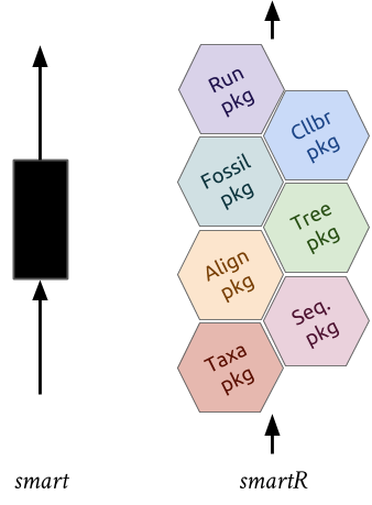
* [`supersmartR`](https://github.com/AntonelliLab/supersmartR) is a series of
R packages that form a phylogenetic pipeline.
* The original [SUPERSMART](https://github.com/naturalis/supersmart) program
uses a "divide-and-conquer" apprach to constructing large phylogenetic trees.
* It combines both a supermatrix (an assembly of multiple gene/clusters into a
single matrix) and a supertree (merging multiple trees) approach.
* `supersmartR` packages are standalone packages with their own functions
and uses BUT they can be combined to recreate the supersmart pipeline.

### [SUPERSMART](http://www.supersmart-project.org/)

![](https://www.ncbi.nlm.nih.gov/pmc/articles/PMC5410925/bin/syw066F1.jpg)

### [supersmartR](https://github.com/AntonelliLab/supersmartR)

![](https://raw.githubusercontent.com/AntonelliLab/supersmartR/master/supersmart%20vs%20supersmartr.png)

## The Workshop

This workshop we will [introduce the packages](#packages) and provide code to
run a simple [pipeline](#pipeline) to create a phylogenetic tree (a supertree
of all Guinea-pig-like species).

* [Introduction to `phylotaR`](#phylotar)
* [Introduction to `restez`](#restez)
* [Introduction to `outsider`](#outsider)
* [Introduction to `gaius`](#gaius)
* [Supertree pipeline](#pipeline)


**Target Duration ~1 hr**

* * *

# Prerequisites

* Software
    * [R](https://cran.r-project.org/) (> 3.5)
    * [RStudio](https://www.rstudio.com/)
    * [Desktop Docker](https://docs.docker.com/install/) (Linux containers)
* Basic knowledge
    * R
    * Phylogenetics

(Windows users may struggle installing Docker Desktop, in which case
[Docker Toolbox](https://docs.docker.com/toolbox/toolbox_install_windows/) will
also work.)

### R packages

Install dependant packages.

```r
# remotes allows installation via GitHub
if (!'remotes' %in% installed.packages()) {
  install.packages('remotes')
}

library(remotes)
# install latest outsider
install_github("antonellilab/outsider.base")
install_github("antonellilab/outsider")
# install latest restez
install_github("hannesmuehleisen/MonetDBLite-R")
install_github("ropensci/restez")
# install latest phylotaR
install_github("ropensci/phylotaR")
# install latest gaius
install_github("antonellilab/gaius")
```

If you're computer is set-up correctly with the R packages and Docker, you
should be able to run the below script without errors (don't worry about
security warnings).

```{r testoutsider, results='hold'}
## Code
library(outsider)
repo <- "dombennett/om..hello.world"
module_install(repo = repo, force = TRUE)
hello_world <- module_import(fname = "hello_world", repo = repo)
hello_world()

## Output

```

* * *

# Setup

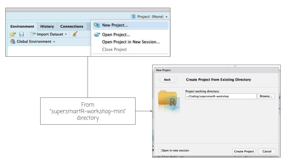
To run all the code in this workshop you will need to:

* Download the zipped folder of this GitHub repo, [click here](https://github.com/AntonelliLab/supersmartR-workshop-mini/archive/master.zip).
* Unzip this folder and place it in a convenient location on your computer (e.g.
"my coding projects").
* Open RStudio and create a new project from this new folder.

![](https://raw.githubusercontent.com/AntonelliLab/supersmartR-workshop-mini/master/assets/rstudio_setup.png)

* * *

# Tutorials

## Packages

### [`phylotaR`](https://github.com/ropensci/phylotaR) <img src="https://raw.githubusercontent.com/ropensci/phylotaR/master/logo.png" height="200" align="right"/>

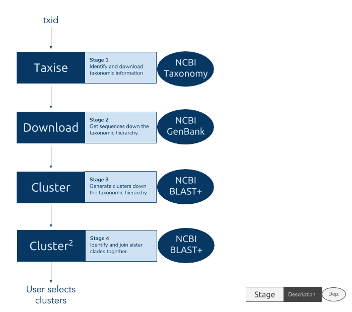
The `phylotaR` package downloads all sequences associated with a given
taxonomic group and then runs all-vs-all BLAST to identify clusters of
sequences suitable for phylogenetic analysis.

The process takes place across four stages:

* Taxise: identify taxonomic IDs
* Download: download sequences
* Cluster: run all-vs-all BLAST
* Cluser^2: run all-vs-all BLAST again

![](https://raw.githubusercontent.com/ropensci/phylotaR/master/other/stages.png)

#### Setup

To run `phylotaR`, we need to set up a folder to host all downloaded files.
Parameters for setting up the folder are provided to the `setup` function.

```{r setup-phylotaR, include=TRUE, eval=FALSE}
# NOT RUN
library(phylotaR)
# available parameters
print(parameters())
# e.g. mnsql = 200 - minimum sequence length
# pass the parameters to the setup() function
# essential parmeters are: wd, txid
wd <- file.path(tempdir(), 'testing_phylotaR')
if (dir.exists(wd)) {
  unlink(x = wd, recursive = TRUE, force = TRUE)
}
dir.create(wd)
setup(wd = wd, txid = '9504', outsider = TRUE, v = TRUE)
# to run the pipeline
# run(wd = wd)
```


#### Parsing results

Read in the phylotaR results with `read_phylota`. But here we will use the
pacakge example data, "Aotus".

##### Summarise the clusters

```{r phylotar-summary-results, echo=TRUE, results='hold'}
library(phylotaR)
data(aotus)
# generate summary stats for each cluster
smmry_tbl <- summary(aotus)
# Important details
#  N_taxa     - number of taxonomic entities associated with sequences in cluster
#  N_seqs     - number of sequences in cluster
#  Med_sql    - median sequence length of sequences in cluster
#  MAD        - measure of the deviation in sequence length of a cluster
#  Definition - must common words in sequence definition lines
smmry_tbl[1:10, ]
```

```{r phylotar-summary-plot}
# plot
p <- plot_phylota_treemap(phylota = aotus, cids = aotus@cids[1:10],
                          area = 'nsq', fill = 'ntx')
print(p)
```

##### Understand the PhyLoTa table (`aotus`)

```{r phylota-table, results='hold'}
# CODE

# PhyLoTa table has ...
# clusters
aotus@clstrs
# sequences
aotus@sqs
# taxonomy
aotus@txdct
# A cluster is a list of sequences
aotus@clstrs@clstrs[[1]]
str(aotus@clstrs@clstrs[[1]])
# A sequence is a series of letters and associated metadata
aotus@sqs@sqs[[1]]
str(aotus@sqs@sqs[[1]])
# A taxonomic record is an ID and associated metadata
txid <- aotus@txids[[1]]
# Information can be extracted from ...
# clusters
get_clstr_slot(phylota = aotus, cid = aotus@cids[1:10], slt_nm = 'nsqs')
# sequences
get_sq_slot(phylota = aotus, sid = aotus@sids[1:10], slt_nm = 'nncltds')
# tax. records
get_tx_slot(phylota = aotus, txid = aotus@txids[1:10], slt_nm = 'scnm')
# Other useful convenience functions
get_nsqs(phylota = aotus, cid = aotus@cids[1:10])
get_ntaxa(phylota = aotus, cid = aotus@cids[1:10], rnk = 'species')

# OUTPUT
```

##### Select clusters

```{r phylotar-selection, results='hold'}
# CODE

# use the summary table to extract cids of interest
nrow(smmry_tbl)
# keep clusters with MAD above 0.5
smmry_tbl <- smmry_tbl[smmry_tbl[['MAD']] >= 0.5, ]
nrow(smmry_tbl)
# keep clusters with more than 10 seqs
smmry_tbl <- smmry_tbl[smmry_tbl[['N_seqs']] >= 10, ]
nrow(smmry_tbl)
# keep clusters with more than 4 species
nspp <- get_ntaxa(phylota = aotus, cid = smmry_tbl[['ID']], rnk = 'species')
selected_cids <- smmry_tbl[['ID']][nspp >= 4]
length(selected_cids)
# create selected PhyLoTa table
selected_clusters <- drop_clstrs(phylota = aotus, cid = selected_cids)

# OUTPUT
```

##### Plotting selected clusters

```{r phylota-plotting, results='hold'}
# CODE

# extract scientific names for taxonomic IDs
scnms <- get_tx_slot(phylota = selected_clusters, txid = selected_clusters@txids,
                     slt_nm = 'scnm')
# plot presence/absence
plot_phylota_pa(phylota = selected_clusters, cids = selected_clusters@cids,
                txids = selected_clusters@txids, txnms = scnms)

```

##### Writing to file

```{r phylota-writeout, results='hold'}
# CODE

# reduce clusters to repr. of 1 seq. per sp.
reduced_clusters <- drop_by_rank(phylota = selected_clusters, rnk = 'species',
                                 n = 1)
reduced_clusters
# write out first cluster
sids <- reduced_clusters@clstrs[['0']]@sids
txids <- get_txids(phylota = reduced_clusters, sid = sids, rnk = 'species')
scnms <- get_tx_slot(phylota = reduced_clusters, txid = txids, slt_nm = 'scnm')
outfile <- file.path(tempdir(), 'cluster_1.fasta')
write_sqs(phylota = reduced_clusters, sid = sids, sq_nm = scnms,
          outfile = outfile)
cat(readLines(outfile), sep = '\n')

# OUTPUT
```

### [`restez`](https://github.com/ropensci/restez) <img src="https://raw.githubusercontent.com/ropensci/restez/master/logo.png" height="200" align="right"/>

`restez` is a package that allows users to download whole chunks of NCBI's
[GenBank](https://www.ncbi.nlm.nih.gov/genbank/). The package works by:

* Downloading compressed files of sections of GenBank
* Unpacking these files and building a local GenBank copy
* Providing generic functions for interacting with the local copy

![](https://raw.githubusercontent.com/ropensci/restez/master/paper/outline.png)

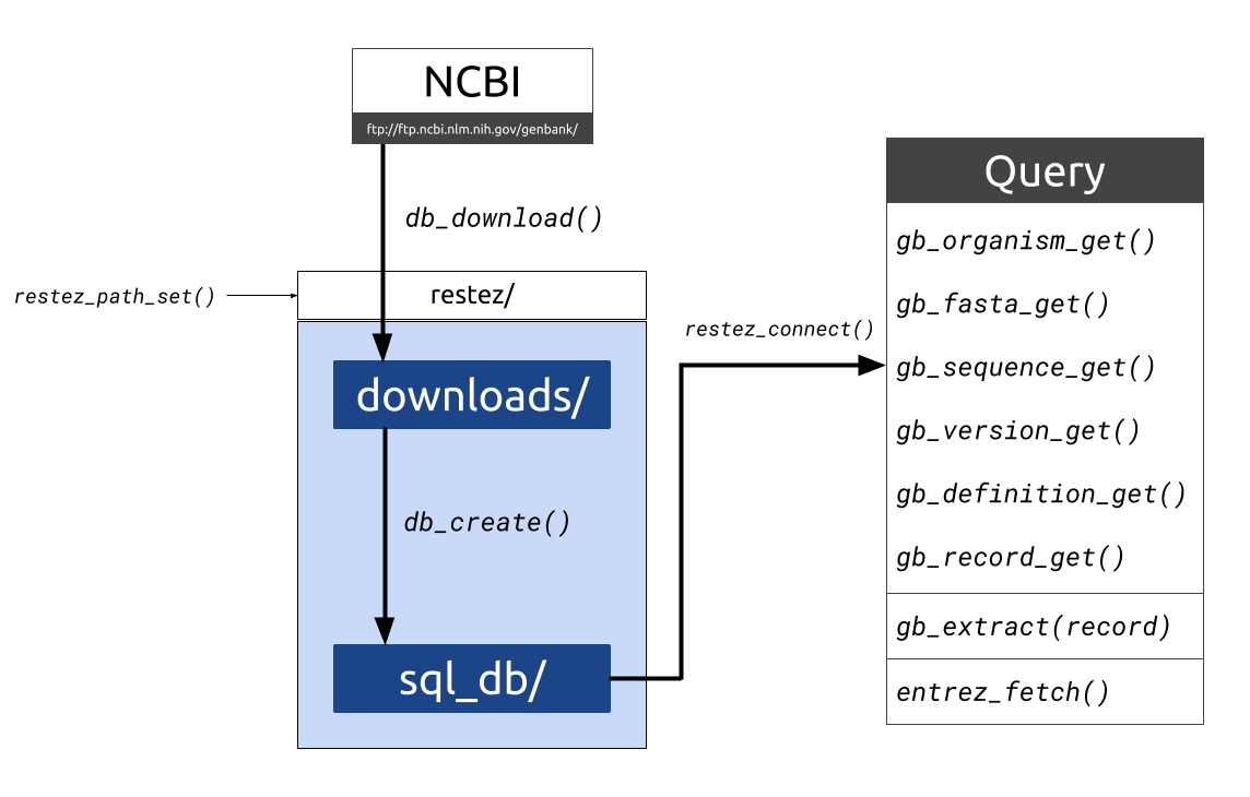
#### Set-up your first `restez` database

Here, we will do the following:

1. Specify a location for our database (`restez_path`)
2. Download the smallest section of GenBank (unannotated)
3. Build a local database

```{r delete-database, include=FALSE}
rstz_pth <- file.path(tempdir(), 'unannotated_database')
if (dir.exists(rstz_pth)) {
  unlink(x = rstz_pth, recursive = TRUE, force = TRUE)
}
```
```{r restez-setup, echo=TRUE, results='hold'}
# CODE

library(restez)
# 1. Set the filepath for where the database will be stored
rstz_pth <- file.path(tempdir(), 'unannotated_database')
if (!dir.exists(rstz_pth)) {
  dir.create(rstz_pth)
}
restez_path_set(filepath = rstz_pth)
# 2. Download
# select number 20, for unannoated (the smallest section)
db_download(preselection = '20')
# 3. Create database
# connect to empty database
restez_connect()
db_create()
# always disconnect from a database when not in use.
restez_disconnect()

# OUTPUT
```

#### Query the database

We can send queries to the database using two different methods: `restez`
functions or [`rentrez`](https://ropensci.org/tutorials/rentrez_tutorial/)
wrappers.

> **What is `rentrez`?** The `rentrez` package allows users to interact with
NCBI Entrez. `restez` wraps around some of its functions so that instead of
sending queries across the internet, the local database is checked first.

```{r querying, echo=TRUE, results='hold'}
# CODE

# import library, point to database and connect
library(restez)
rstz_pth <- file.path(tempdir(), 'unannotated_database')
restez_path_set(filepath = rstz_pth)
restez_connect()
# Check the status
restez_status()
# Get a random ID from the database
id <- sample(x = list_db_ids(n = 100), size = 1)
# print record information
record <- gb_record_get(id)
cat(record)
# see ?gb_record_get for more query functions
# always disconnect
restez_disconnect()

# OUTPUT
```

### [`outsider`](https://github.com/antonellilab/outsider) <img src="https://raw.githubusercontent.com/antonellilab/outsider/master/logo.png" height="200" align="right"/>

`outsider` is a package that allows users to install and run external code
within the R environment. This is very useful when trying to construct
pipelines that make use of a variety of code. `outsider` requires Docker to
work. It should be able to launch any (?!) command-line program.

![](https://raw.githubusercontent.com/AntonelliLab/outsider/master/other/outline.png)

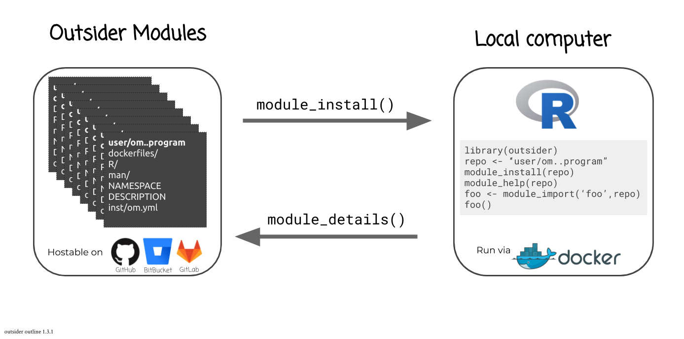
You can find out what modules are available for a given coding-service using:

```{r outsider-available, echo=TRUE, results='hold'}
library(outsider)
module_details(service = 'github')
```

There is also a package called
["outsider.devtools"](https://github.com/AntonelliLab/outsider.devtools) that
makes it easier to create your own moduules, see `other/outsider_devtools.R`

#### Running alignment software

To demonstrate, let's run an alignment software tool,
[mafft](https://mafft.cbrc.jp/alignment/software/), from within R. Let's
install a module for mafft, and then run it on some test sequences
("ex_seqs.fasta").

#### Install

```{r remove-mafft, include=FALSE}
if (outsider::is_module_installed('dombennett/om..mafft')) {
  outsider::module_uninstall('dombennett/om..mafft')
}
```

```{r outsider-mafft, echo=TRUE, results='hold'}
# CODE

library(outsider)
# squelch text to console
verbosity_set(show_program = FALSE, show_docker = FALSE)
# github repo to where the module is located
repo <- 'dombennett/om..mafft'
# install mafft
module_install(repo = repo, force = TRUE)
# look up available functions
(module_functions(repo = repo))
# import mafft function
mafft <- module_import(fname = 'mafft', repo = repo)
# test function
mafft(arglist = '--help')

# OUTPUT
```

#### Align

```{r outsider-align, echo=TRUE, results='hold'}
library(outsider)
# Use example mafft nucleotide data
ex_seqs_file <- file.path(getwd(), 'data', 'ex_seqs.fasta')
(file.exists(ex_seqs_file))
# Run
mafft <- module_import(fname = 'mafft', repo = 'dombennett/om..mafft')
ex_al_file <- file.path(getwd(), 'data', "ex_al.fasta")
mafft(arglist = c('--auto', ex_seqs_file, '>', ex_al_file))
(file.exists(ex_al_file))
# View alignment
cat(readLines(con = ex_al_file, n = 50), sep = '\n')
```

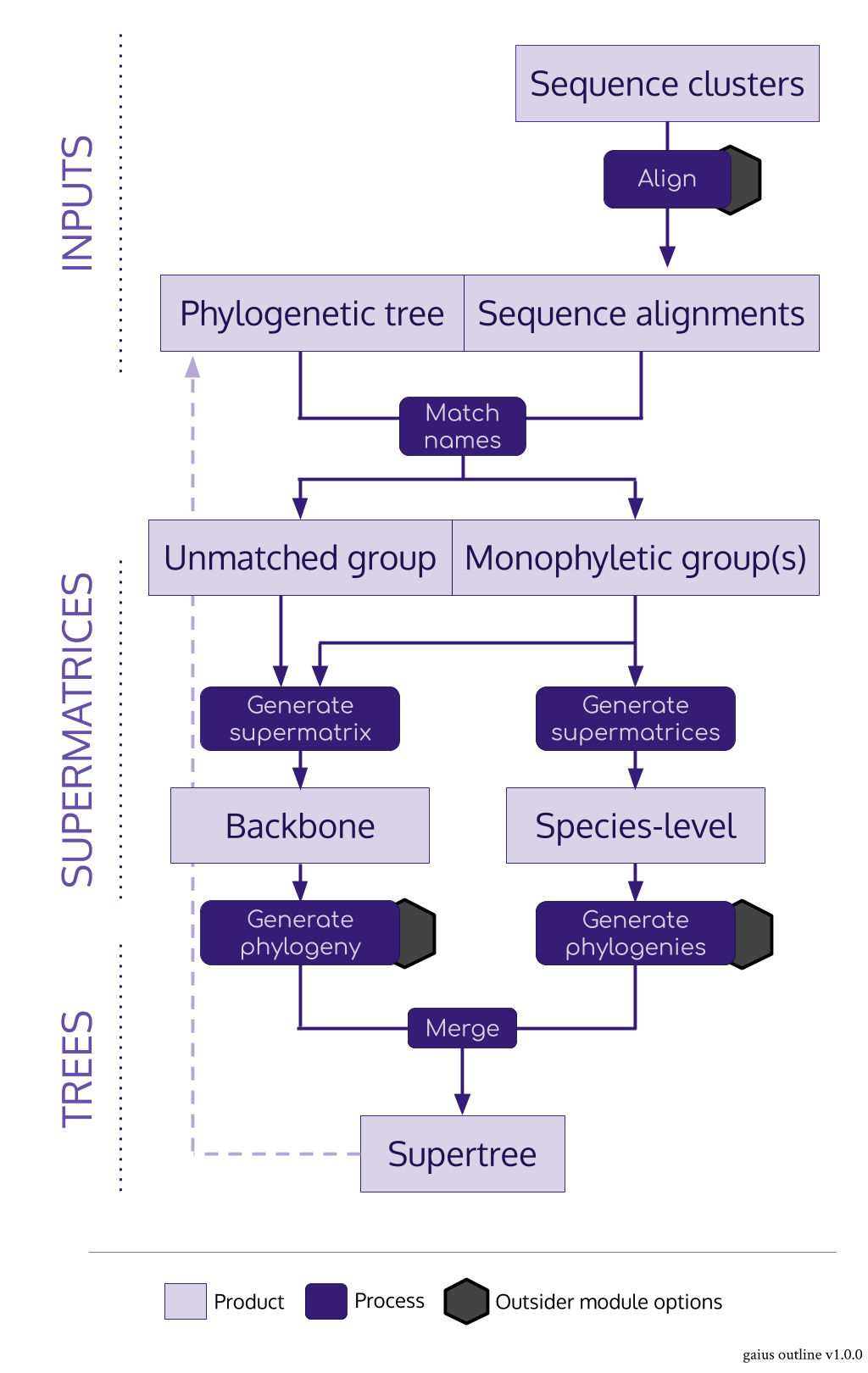
### [`gaius`](https://github.com/antonellilab/gaius) <img src="https://raw.githubusercontent.com/antonellilab/gaius/master/logo.png" height="200" align="right"/>

* `gaius` acts as the nexus package for the SUPERSMART pipeline in R
* It imports both alignments and trees and produces supermatrices and
supertrees
* Its main role is to identify monophyletic groups of a given number of taxa
for species-level trees
* The main "trick" is to use a pre-existing tree
* It can do a few clever things: there can be any number of levels of backbone,
backbone supermatrices are constucted from an assortment of the best
monophyletic sequences

![](https://raw.githubusercontent.com/AntonelliLab/gaius/master/other/outline.png)

```{r gaius, results='hold'}
# CODE

library(gaius)
# vars
alignment_dir <- file.path(getwd(), 'data', 'gaius_alignments')
tree_file <- file.path(getwd(), 'data', 'taxtree.tre')
# alignment files
alignment_files <- file.path(alignment_dir,
                             list.files(path = alignment_dir,
                                        pattern = '.fasta'))
(alignment_files[1:2])
# get alignment names
alignment_names <- names_from_alignments(alignment_files)
(alignment_names[1:10])
# tree tip names
tree_names <- names_from_tree(tree_file)
(tree_names[1:10])
# match alignment names to those in tree
matched_names <- name_match(alignment_names = alignment_names,
                            tree_names = tree_names)
(matched_names)
# identify monophyletic groups
groups <- groups_get(tree_file = tree_file, matched_names = matched_names)
(groups)
# read in alignments
alignment_list <- alignment_read(flpths = alignment_files)
(alignment_list)
# ^ for a better idea of the alignment, try ...
# viz(alignment_list[[1]])
# construct supermatrices
supermatrices <- supermatrices_get(alignment_list = alignment_list,
                                   groups = groups, min_ngenes = 2,
                                   min_ntips = 3, min_nbps = 100,
                                   column_cutoff = 0, tip_cutoff = 0.1)
(supermatrices)

# OUTPUT
```


## Pipeline

![](https://raw.githubusercontent.com/AntonelliLab/supersmartR-workshop-mini/master/assets/cavvy_shot.png)

A complete pipeline for constructing a phylogenetic tree of all Caviomorpha
species is contained in `pipeline/`. The pipeline uses the above packages and their functions. We can run each script of the pipeline using `source()`. (To
save time we will skip the `restez` and `phylotaR` steps and download a
completed folder of the first part of the results.)

```{r pipeline, results='hold'}
## Code

# minor outsider set-up
if (file.exists('gc_setup.R')) {
  source(file = 'gc_setup.R', local = FALSE, echo = FALSE, print.eval = FALSE)
} else {
  threads <- 4
}

# save time by skipping the first two stages by using the ready
#  1_phylotaR/ in data/
zipfile <- file.path('data', '1_phylotaR.zip')
if (file.exists(zipfile)) {
  utils::unzip(zipfile = zipfile, exdir = 'pipeline', overwrite = TRUE)
}

# run each script in the pipeline
stage_scripts <- c('2_clusters.R', '3_align.R', '4_supermatrix.R',
                   '5_phylogeny.R', '6_supertree.R', '7_view.R')
start_time <- Sys.time()
cat('Running pipeline ....\n', sep = '')
for (stage_script in stage_scripts) {
  cat('... ', crayon::green(stage_script), '\n', sep = '')
  scriptenv <- new.env()
  scriptenv$threads <- threads
  suppressMessages(source(file.path('pipeline', stage_script),
                          local = scriptenv, echo = FALSE, print.eval = FALSE))
}
end_time <- Sys.time()
duration <- difftime(end_time, start_time, units = 'mins')
cat('Duration: ', crayon::red(round(x = duration, digits = 3)), ' minutes.\n')

# clear-up
outsider::ssh_teardown()

## Output
```

The resulting tree consists of 185 tips, generating from 16 gene/clusters.

![supertree](supertree.png)

***

**Learn more: [`supersmartR` GitHub Page](https://github.com/AntonelliLab/supersmartR)**