The dataset that we have chosen to use for this assignment is the diamonds Dataset that is available as a built-in dataset in the ggplot2 package in R and was accessed through Tidyverse’s official GitHub repository of raw datasets for ggplot2. The original source of this dataset is from the Loose Diamonds Search Engine website (Fairfield County Diamonds, Inc., n.d.).
Dataset Source Link: https://github.com/tidyverse/ggplot2/blob/main/data-raw/diamonds.csv
This dataset contains 53940 rows of data and 10 variables which are Carat, Cut, Colour, Clarity, Depth, Table, Price, x, y, and z. Carat describes the weight of the diamond, Cut describes the cut quality of the diamond graded by Fair, Good, Very Good, Premium, Ideal, Colour describes the colour of the diamond where D is the best colour and J is the worst, Clarity describes how clear the diamond is, it is graded by I1, SI2, SI1, VS2, VS1, VVS2, VVS1, IF, where I1 is the worst and IF is the best. For example, l1 means “level 1 Included”, FL means “Flawless”, VS means “Very Slightly Included”, VVS means “Very Very Slightly Included”, and so on. Depth (depthPercent) describes the height of a diamond, measured from the culet to the table, divided by its average girdle diameter. Table is the width of the diamond's table expressed as a percentage of its average diameter, Price is the price of the diamond in US dollars, x (length) is the length of the diamond in millimetres, y (width) is the width of the diamond in millimetres, and z (depth) is the depth of the diamond in millimetres. The variables carat, depth, table, price, x, y, and z are continuous variables whereas cut, colour, and clarity are categorical ordinal variables in this dataset.
The analysis objectives of this assignment using the diamonds dataset are to identify trends and patterns from the data and to predict the price of diamonds based on the other features in this dataset. SAS Studio is used as the SAS programming interface for this project.
Before performing statistical modelling and analysis on our dataset, it is necessary to deploy descriptive analysis to better understand and get an overview of the dataset.

As shown in Figure 1, we observed the output table that lists out the variables of our dataset as well as the data type that was interpreted by SAS studio. As expected, the data type of variable cut, colour and clarity are character data types (char) whereas all the other variables are in numeric data (num).
In view that we are interested in using a multiple linear regression model to predict the price of diamonds and linear regression model requires all input variables to be numeric, we encoded the variables cut, colour and clarity are ordinal categorical variables to numeric variables. As shown in Figure 2, the values of cut variable Fair, Good, Very Good, Premium and Ideal are encoded to the numbers 1 to 5 respectively; the values of color variable J, I, H, G, F, E and D are encoded to the numbers 1 to 7 respectively; the values of clarity variable SI2, SI1, VS2, VS1, VVS2, VVS1, IF are encoded to the numbers 1 to 8 respectively. The encoded variables cut, color and clarity are then assigned to new columns namely cutNo, colorNo and clarityNo.


Figure 3 displays the summary statistics of all 10 numeric variables that were interpreted by SAS studio. The mean price of the diamond is $3932.80, and the minimum and maximum price of the diamonds are $326.00 and $18823.00. The standard deviation of price is $3989.44, which is very close to the mean price, meaning that the data is centered around the mean, and data points are less dispersed. Furthermore, the mean carat of the diamond is 0.80 with minimum and maximum values of 0.20 and 5.01 carats respectively. The standard deviation of carat is 0.47, which is relatively far to the mean carat value, meaning that the data points are quite dispersed. This shows that the carat of diamonds in the dataset have a significant difference. Besides that, the mean of the variable table is 57.46%, with minimum and maximum values of 43.00% and 95.00% respectively. The standard deviation of the variable table is 2.23%, which is very far from the mean table percentage, meaning that the data points are very dispersed among each other. It is also observed that the minimum value of length, width and depth variables are 0, this suggests that there might be some faulty data in the dataset that should be cleaned. The table shows that there are no missing values in this dataset.
After observing the summary statistics which shows the basic statistical measures such as the mean, median, range, standard deviation, minimum and maximum of the variables, we examined the frequency table (Figure 4) for variable cutNo colorNo and clarityNo

Next, we are interested in checking the normality assumption on the continuous variables carat, depth, table, price, x, y, and z. As shown in Figure 5, the Q-Q plot for each continuous variable is generated and examined. It is suggested that the residuals of all variables excluding the variable price do not significantly violate the normality assumption. The variable price is not normally distributed. According to a research by Li et al. (2012), linear regression is appropriate for analysis when dependent variable is not distributed normally given that dataset has a large sample size (>3000). However, we shall still consider the removal of high leverage points or outliers that are potential influential points and data transformation methods.

To identify outliers, the distribution plot and box plot of each variable is examined to understand the value distribution for each continuous variable (Figure 6). By observing the boxplots, it is apparent that all variables have some outliers. Therefore, it was necessary to deploy data cleaning techniques to remove outliers. Observations that have a value of 0 are removed for variables length, width and depth. Depthpercent that has values below 45 or 75 and table that has values above 90 is also deleted (Figure 7).


Before performing statistical modelling to predict the price of diamonds based on the other variables in this dataset, a scatter plot matrix is constructed to investigate the linear relationships between variables and to check for outliers. As seen in Figure 8, all 7 continuous variables are plotted against each other. It is observed that variable width and depth have a strong correlation with price; variable carat and length have a moderate correlation with price; variable depthPercent and table does not have a significant relation with price. It is also observed that there still remain some outliers that would be considered for removal.

After that, a multiple linear regression model is constructed to have an overview of the model performance in predicting the price of diamonds based on all other variables in this dataset. The output result of the regression model is shown in Figure 9. It is observed that our model has an R-Square value and Adjusted R-Square of 0.9070. Therefore, 90.7% of the variation in diamond price is explained by the variation in carat, cutNo, colorNo, clarityNo, depthpercent, table, length, width and depth. However, the variance inflation factors values suggest that there might be a collinearity problem in the model since the VIF is larger than 10 for variable carat, length, width and depth.
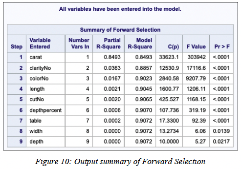
To justify the choice of our multiple linear regression model, we performed the model selection procedure such as forward selection, backward elimination and stepwise selection to select the most suitable model for this dataset. As shown in Figure 10, 11 and 12, all three model selection methods produced an output that suggests the input of all variables into the regression model is the model that best fits the observed data.


In addition, the Mallows’ Cp values are also computed for each possible model combination to find the best model for this dataset. The best 20 models that have the lowest Cp values are shown in Figure 13. Figure 14 shows the Cp values for the best 20 models (represented by the dots and stars) versus the number of parameters in the fitted model. By observing Figure 14, the smallest model with an observation below both the Mallows and Hocking line has p = 10. Hence, we know that there are 9 explanatory variables for this chosen model. In other words, the model with all variables is the best model based on both Mallows and Hocking criteria.


After performing model selection, it was necessary to deploy regression diagnostics to ensure that the standard regression assumptions are satisfied. Regression Diagnostics plots such as Studentized Deleted Residuals (RStudent) plot, Cook’s Distance (Cook’s D) plot, Difference in Fit (DFFit) plot and Difference in Beta (DFBeta) plot is generated to identify high leverage points and outliers that are potential influential data. Based on Figure 15, the RStudent plot shows a significant number of observations beyond two standard errors from the mean of 0. The Cook’s D plot and DFFit plot shows that there are several potential influential observations in the dataset, particularly observation #48411 and #24068. Based on the DFBeta plot, observation #48411 is influential because of its effects on depthpercent, length and depth whereas #24068 is influential because of its effects on width.

In Figure 16, observations #48411 and #24068 are printed out to verify if they are faulty data that should be removed. For observation #24068, the value of width is 58.90, which is highly unusual (outlier) because variable width has a mean value of 5.73 based on Figure 3. For observation #48411, the value of depth is 31.80, which is also highly unusual (outlier) because variable depth has a mean value of 3.54 based on Figure 3. It has been verified that both observations #48411 and #24068 are faulty data that should be removed from the dataset.

After that, the 4 regression diagnostics plots are generated again to identify if high leverage points and outliers that are potential influential data still exist in the dataset. The process of identifying and verifying if influential points are faulty data iterates until most significant influential points that may affect the performance of the regression model are identified. Figure 17 shows another 5 influential points that were identified, each influential points were verified to ensure that they are faulty data before being removed. For observation #49190, the value of width is 31.80, which is abnormal (outlier) because variable width has a mean value of 5.73 based on Figure 3. However, observation #27416, #20695, #14636 and #21655 does not have any unusual data within the observation. Therefore, only observation #49190 is removed from the dataset.

After performing model selection and model diagnostics that lead to the removal of several influential points that had been verified as faulty data, another multiple linear model regression model is constructed. The output of the new model is shown in Figure 18.

Based on Figure 18, there are now 53910 numbers of observations. The output results of the new regression model in Figure 18 were interpreted and analysed. It is observed that our updated model has an R-Square value and Adjusted R-Square of 0.9077. Therefore, 90.77% of the variation in diamond price is explained by the variation in carat, cutNo, colorNo, clarityNo, depthpercent, table, length, width and depth. Furthermore, around 90.77% of the variation in diamond price can be explained by the variation in carat, cutNo, colorNo, clarityNo, depthpercent, table, length, width and depth, adjusted by number of predictors and sample size. R-Square value and Adjusted R-Square of this new regression model have slightly improved as compared to the previous model in Figure 9. The coefficient of variation is 30.82, which is relatively low, this suggests a good model fit. However, the variance inflation factors values suggest that there might be a collinearity problem in the model since the VIF is larger than 10 for variable carat, length, and width.

𝐻0: There is no linear relationship between the response variable and the explanatory variables.
𝐻1: There is a linear relationship between the response variable and at least one of the explanatory variables.
To determine the collective influence of the explanatory variables in this dataset it is required to perform an overall F-test that is used in the hypothesis testing procedure. Based on Figure 18, the F-value is 66237.1 and the p-value is <0.0001. The p-value is < 0.0001, thus null hypothesis is rejected at the 0.05 level of significance (𝛼 = 0.05). Therefore, at least one of the explanatory variables has a significant effect on the response variable.
Inference for Individual Regression Coefficients and Confidence Interval Estimate for the Slope Next, a test for the significance of the individual regression coefficients is needed to determine which explanatory variables have a significant effect on the response variable.

where 𝛽1 is the partial regression coefficient for 𝑋1 (carat).
The test statistic t-value for carat is 198.43 with corresponding p-value is < 0.0001, null hypothesis is rejected at significance level 𝛼 = 0.05. There is strong evidence that carat is related to the price, controlling for the other variables.
Controlling for other explanatory variables in the model, we are 95% confident that the change in the mean price per weight (g) increase in carat falls between $10802 and $11018.

Where 𝛽2 is the partial regression coefficient for 𝑋2 (cutNo).
The test statistic t-value for cutNo is 22.34 with corresponding p-value is < 0.0001, null hypothesis is rejected at significance level 𝛼 = 0.05. There is strong evidence that cutNo is related to the price, controlling for the other variables.
Controlling for other explanatory variables in the model, we are 95% confident that the change in the mean price per diamond quality increase in cutNo falls between $117.04 and $139.55.

Where 𝛽3 is the partial regression coefficient for 𝑋3 (colorNo).
The test statistic t-value for colorNo is 99.30 with corresponding p-value is < 0.0001, null hypothesis is rejected at significance level 𝛼 = 0.05. There is strong evidence that colorNo is related to the price, controlling for the other variables.
Controlling for other explanatory variables in the model, we are 95% confident that the change in the mean price per diamond color increase in colorNo falls between $316.08 and $328.81.

Where 𝛽4 is the partial regression coefficient for 𝑋4 (clarityNo).
The test statistic t-value for clarityNo is 140.16 with corresponding p-value is < 0.0001, null hypothesis is rejected at significance level 𝛼 = 0.05. There is strong evidence that clarityNo is related to the price, controlling for the other variables.Controlling for other explanatory variables in the model, we are 95% confident that the change in the mean price per diamond clarity increase in clarityNo falls between $486.37 and $501.19.

Where 𝛽5 is the partial regression coefficient for 𝑋5 (depthpercent).
The test statistic t-value for depthpercent is -17.91 with corresponding p-value is < 0.0001, null hypothesis is rejected at significance level 𝛼 = 0.05. There is strong evidence that depthpercent is related to the price, controlling for the other variables.
Controlling for other explanatory variables in the model, we are 95% confident that the change in the mean price per diameter increase in depthpercent falls between

Where 𝛽6 is the partial regression coefficient for 𝑋6 (table).
The test statistic t-value for table is -6.69 with corresponding p-value is < 0.0001, null hypothesis is rejected at significance level 𝛼 = 0.05. There is strong evidence that the variable table is related to the price, controlling for the other variables.
Controlling for other explanatory variables in the model, we are 95% confident that the change in the mean price per diamond increase in table (width of the diamond's table expressed as a percentage of its average diameter) falls between

Where 𝛽7 is the partial regression coefficient for 𝑋7 (length).
The test statistic t-value for length is -26.09 with corresponding p-value is < 0.0001, null hypothesis is rejected at significance level 𝛼 = 0.05. There is strong evidence that length is related to the price, controlling for the other variables.
Controlling for other explanatory variables in the model, we are 95% confident that the change in the mean price per millimeters increase in length falls between

Where 𝛽8 is the partial regression coefficient for 𝑋8 (width).
The test statistic t-value for width is 16.55 with corresponding p-value is < 0.0001, null hypothesis is rejected at significance level 𝛼 = 0.05. There is strong evidence that width is related to the price, controlling for the other variables.
Controlling for other explanatory variables in the model, we are 95% confident that the change in the mean price per millimeters increase in width falls between $1352.69 and $1716.17.
It is concluded that all variables namely carat, cutNo, colorNo, clarityNo, depthpercent, table, length, width and depth has a significant effect on the response variable.